
Thanks, the issue might be character-related: Could you do the same thing, but this time, where the code says
delim = '-'
replace the '-' by copying an pasting the hyphen from the console that you see bewteen 2010 and 05 and then rerun the code and screenshot again?
Thank you so much for your time with this, I really appreciate it. I have copied and pasted the screenshot from the console and reran the code but am getting the same error.
OK, a final try then for the day — note I'm not using read.csv(), but read_csv():
data <- read_csv("fifteenminuteintervaldata.csv")
data |>
  separate_wider_delim(
    cols = Date,
    names = c("year", "month", "day"),
    delim = '-',
    cols_remove = F) |>
  group_by(year, month) |>
  summarise(
    Precipitation = sum(Precipitation),
    Discharge = sum(Discharge)
  ) |>
  dput()
Thank you, here is my output
dput()
`summarise()` has grouped output by 'year'. You can override using the `.groups` argument.
structure(list(year = c("2010", "2010", "2010", "2010", "2010",
"2010", "2011", "2011", "2011", "2011", "2011", "2011", "2012",
"2012", "2012", "2012", "2012", "2012", "2013", "2013", "2013",
"2013", "2013", "2013", "2014", "2014", "2014", "2014", "2014",
"2014", "2015", "2015", "2015", "2015", "2015", "2015", "2016",
"2016", "2016", "2016", "2016", "2016", "2017", "2017", "2017",
"2017", "2017", "2017", "2018", "2018", "2018", "2018", "2018",
"2018", "2019", "2019", "2019", "2019", "2019", "2019", "2020",
"2020", "2020", "2020", "2020", "2020", "2021", "2021", "2021",
"2021", "2021", "2021", "2022", "2022", "2022", "2022", "2022",
"2022", NA), month = c("05", "06", "07", "08", "09", "10", "05",
"06", "07", "08", "09", "10", "05", "06", "07", "08", "09", "10",
"05", "06", "07", "08", "09", "10", "05", "06", "07", "08", "09",
"10", "05", "06", "07", "08", "09", "10", "05", "06", "07", "08",
"09", "10", "05", "06", "07", "08", "09", "10", "05", "06", "07",
"08", "09", "10", "05", "06", "07", "08", "09", "10", "05", "06",
"07", "08", "09", "10", "05", "06", "07", "08", "09", "10", "05",
"06", "07", "08", "09", "10", NA), Precipitation = c(41.6, 63.4,
30.4, 58, 109.2, 38, 4, 62.6, 67.8, 30.8, 39, 34.2, 140.2, 94.6,
51, 104.2, 29.8, 40.2, 142.2, 55.2, 126.6, 50.8, 9.8, 37, 57.2,
109, 22.6, 39.8, 6.6, 14.4, 95.6, 66.8, 34.4, 77.2, 44, 48, 47.8,
102.2, 79.4, 43, 24.2, 0, 72.2, 70, 60.6, 70, 81.4, 36.8, 53.8,
71.2, 77.8, 42.8, 79, 102.4, 43.4, 73, 64.2, 61.4, 100.6, 89.6,
102, 12.2, 5, 81, 49.4, 64.8, 47, 72.6, 12.4, 33.4, 60.4, 50.6,
100.4, 67.4, 52.4, 33, 99.2, 25.2, NA), Discharge = c(1098.165,
913.832, 143.449, 122.327, 628.503, 744.365, 3576.262758593,
1169.660438716, 636.443304331, 89.993293314, 87.987612867, 156.547529614,
3135.631004576, 2642.972454083, 247.869505193, 184.387420593,
72.984364263, 144.809074076, 7140.468275454, 1947.160139933,
3472.148888357, 827.989476767, 1169.288358022, 830.330769324,
7099.102561831, 3781.54435038, 1403.538744855, 477.311791977,
415.568367489, 347.669041685, 2712.445233732, 1453.426870664,
598.906750422, 336.028010752, 684.973451554, 590.387748128, 1969.451711015,
3125.837815424, 1722.36845952, 271.31683909, 503.568190585, 740.808522966,
4398.121089032, 1678.901533343, 1080.74882027, 302.582297029,
1017.53118285, 1286.086914624, 1958.065068929, 939.237816557,
1289.604132466, 163.11710896, 445.258625216, 1813.391561568,
4093.504092264, 2022.328847569, 582.173185702, 286.591893656,
1466.749048724, 3481.635663176, 2094.152961024, 642.646409983,
521.921978323, 363.166217808, 395.686164598, 831.226330386, 2097.401490171,
1233.149951321, 154.346937294, 110.370471482, 196.085973386,
415.034224673, 12515.462389965, 2910.924209312, 770.455482982,
450.402574557, 821.166584692, 503.228680048, 0.275960889)), class = c("grouped_df",
"tbl_df", "tbl", "data.frame"), row.names = c(NA, -79L), groups = structure(list(
    year = c("2010", "2011", "2012", "2013", "2014", "2015",
    "2016", "2017", "2018", "2019", "2020", "2021", "2022", NA
    ), .rows = structure(list(1:6, 7:12, 13:18, 19:24, 25:30,
        31:36, 37:42, 43:48, 49:54, 55:60, 61:66, 67:72, 73:78,
        79L), ptype = integer(0), class = c("vctrs_list_of",
    "vctrs_vctr", "list"))), class = c("tbl_df", "tbl", "data.frame"
), row.names = c(NA, -14L), .drop = TRUE))```There must a bug somewhere to chase down, but this is very helpful. I'll can't continue now, but will post again later.
Ok, thank you so much for your time today. I really appreciate it.
I just wanted to let everyone know, I have adjusted my plot and now have the dates properly labelled. I broke the plot down into 13 separate plots (one for each year between 2010 and 2022).
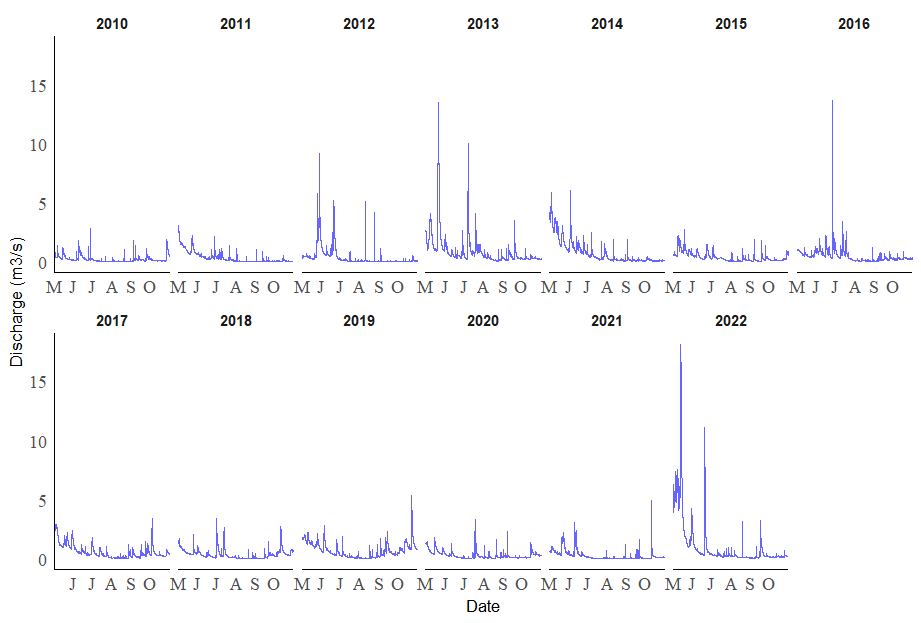
Here is my working code if anyone is interested
# Step 1: Load the Data
library(readr)
library(dplyr)
library(lubridate)
library(ggplot2)

# Load the data
data <- read_csv("fifteenminuteintervaldata.csv")

# Load the data
data <- read_csv("fifteenminuteintervaldata.csv")

# Remove rows with missing or invalid Date or Time values
clean_data <- data %>%
  filter(!is.na(Date) & !is.na(Time))

# Prepare the data
clean_data <- clean_data %>%
  mutate(DateTime = ymd_hms(paste(Date, Time)),
         Year = year(DateTime),
         Month = month(DateTime),
         Day = day(DateTime))

# Filter data for May 1 to October 31 for each year
filtered_data <- clean_data %>%
  filter(Month >= 5 & Month <= 10)

# Define custom function for date labels
custom_month_labels <- c("M", "J", "J", "A", "S", "O")

# Plotting
ggplot(filtered_data, aes(x = DateTime, y = Discharge, group = Year)) +
  geom_line(color = "blue", alpha = 0.6, lwd = 0.01) +
  labs(x = "Date", y = "Discharge (m3/s)") +
  theme_minimal() +
  theme(axis.text = element_text(family = "Times New Roman", size = 12),
        panel.grid.major = element_blank(),
        panel.grid.minor = element_blank(),
        axis.line = element_line(color = "black"),
        strip.background = element_blank(),
        strip.text.x = element_text(size = 10, face = "bold")) +
  scale_x_datetime(date_breaks = "1 month", date_labels = custom_month_labels, expand = c(0, 0)) +
facet_wrap(~ Year, scales = "free_x", nrow = 2)```Good to see! And it looks like you have the tools to what you originally set out to do, too, so to confirm — I assume you have no need of help with your original question,right? And just one comment:
ggplot() removes NA's automatically, so no need to filter out rows with them.
Yes, I believe that I have everything that I need now and no longer need help with my original question. Thank you so much for your help.
Actually, I do have one quick question. The 13 plots that I have created show discharge as a continuous line graph for each year between 2010 and 2022. I also wish to create a series of 13 bar plots (similar to the plots above, but bar plots) showing precipitation depth. Does anyone have any advice on how to adjust this code to create a similar arrangement of plots, but using a bar plot instead of a line plot?
The easiest tweak to make would be to replace geom_line() with geom_col(); you would just need to remove the lwd argument you used with geom_line().
Great. Thank you so much. That worked.
This topic was automatically closed 21 days after the last reply. New replies are no longer allowed.
If you have a query related to it or one of the replies, start a new topic and refer back with a link.