Holts Method forecast model

[andre92]

Hey,

I am trying to use the holt command to forecast some data that I have. I have only 100 observations. However, when I tried to use the command the forecast was not good.

Here is my code:

p2_holts <- holt(ts_p3, h = 12)
plot(p2_holts)

[EconProf]

Please explain what you mean by not good. A reprex would be helpful.

[andre92]

@EconProf

reprex

**

**

Holt's Method

fit23 <- holt(ts_p2, h = 12)
p2_holts <- forecast(fit23, h = 12)
plot(p2_holts)

I want to improve my graph

[arthur.t]

I don't see anything wrong or unusual about the forecast.

You can try ets instead of holt. I believe ets will attempt to detect and include seasonality, while holt will not.

[arthur.t]

Perhaps worth pointing out that it's the seasonality specifically that causes an ets forecasts to be "wiggly."

If there is no seasonality detected, the forecast will be a straight line. At least most of the time. Perhaps there could be a slight curve at the beginning due to interaction of trend and level?

Perhaps it's underwhelming, but you can think of ets as drawing the straight line with the best slope / intercept as possible. If there's no seasonality, then past fluctuations were quite possibly noise, and there's no relevant information to carry forward to inform a wiggle.

[EconProf]

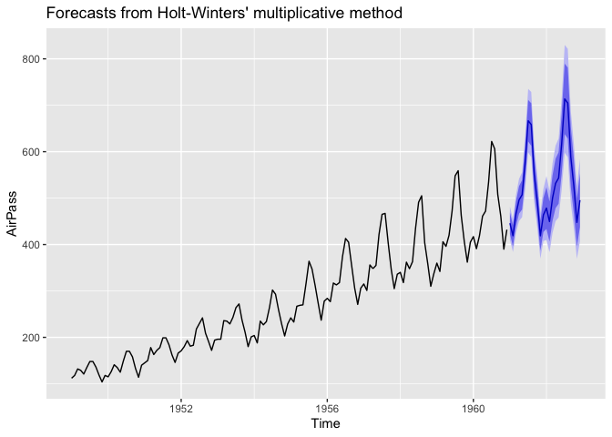
The ups and downs do not appear to follow a consistent seasonal pattern, so exponential smoothing will just average them out. Still, you could try Holt-Winters using hw() from the same {forecast} package as holt(). I would suggest setting seasonal = "multiplicative" in hw(). The seasonal variation is increasing as an amount but may be stable as a percentage (multiple).

[EconProf]

This is an example reprex using the AirPassengers data from the {datasets} package in base R.

I ran dput(AirPassengers) and pasted the output into an RScript, adding "AirPass <-" at the start of the first line, then the rest of the code and created the reprex. This can be very useful for someone trying to help you.

library(forecast)
#> Registered S3 method overwritten by 'quantmod':
#>   method            from
#>   as.zoo.data.frame zoo
AirPass <- structure(c(112, 118, 132, 129, 121, 135, 148, 148, 136, 119, 
            104, 118, 115, 126, 141, 135, 125, 149, 170, 170, 158, 133, 114, 
            140, 145, 150, 178, 163, 172, 178, 199, 199, 184, 162, 146, 166, 
            171, 180, 193, 181, 183, 218, 230, 242, 209, 191, 172, 194, 196, 
            196, 236, 235, 229, 243, 264, 272, 237, 211, 180, 201, 204, 188, 
            235, 227, 234, 264, 302, 293, 259, 229, 203, 229, 242, 233, 267, 
            269, 270, 315, 364, 347, 312, 274, 237, 278, 284, 277, 317, 313, 
            318, 374, 413, 405, 355, 306, 271, 306, 315, 301, 356, 348, 355, 
            422, 465, 467, 404, 347, 305, 336, 340, 318, 362, 348, 363, 435, 
            491, 505, 404, 359, 310, 337, 360, 342, 406, 396, 420, 472, 548, 
            559, 463, 407, 362, 405, 417, 391, 419, 461, 472, 535, 622, 606, 
            508, 461, 390, 432), .Tsp = c(1949, 1960.91666666667, 12), class = "ts")

fit <- hw(AirPass, seasonal = "multiplicative")
summary(fit)
#> 
#> Forecast method: Holt-Winters' multiplicative method
#> 
#> Model Information:
#> Holt-Winters' multiplicative method 
#> 
#> Call:
#>  hw(y = AirPass, seasonal = "multiplicative") 
#> 
#>   Smoothing parameters:
#>     alpha = 0.3146 
#>     beta  = 0.0071 
#>     gamma = 0.5977 
#> 
#>   Initial states:
#>     l = 120.3796 
#>     b = 1.7757 
#>     s = 0.9298 0.7946 0.9024 1.0451 1.1338 1.1388
#>            1.0529 0.9638 1.0349 1.0807 0.9854 0.9378
#> 
#>   sigma:  0.0407
#> 
#>      AIC     AICc      BIC 
#> 1405.654 1410.511 1456.141 
#> 
#> Error measures:
#>                    ME     RMSE      MAE       MPE     MAPE      MASE      ACF1
#> Training set 1.256973 10.63256 7.790649 0.2182707 2.914411 0.2432275 0.2135914
#> 
#> Forecasts:
#>          Point Forecast    Lo 80    Hi 80    Lo 95    Hi 95
#> Jan 1961       445.8901 422.6577 469.1225 410.3592 481.4210
#> Feb 1961       418.9478 396.0288 441.8667 383.8963 453.9993
#> Mar 1961       466.4298 439.7182 493.1414 425.5780 507.2816
#> Apr 1961       496.1291 466.4627 525.7955 450.7583 541.4999
#> May 1961       507.1463 475.5546 538.7381 458.8309 555.4617
#> Jun 1961       575.6281 538.3478 612.9083 518.6129 632.6432
#> Jul 1961       666.6573 621.8494 711.4652 598.1295 735.1850
#> Aug 1961       658.4970 612.6386 704.3554 588.3627 728.6313
#> Sep 1961       550.0907 510.4559 589.7255 489.4745 610.7069
#> Oct 1961       491.7130 455.1069 528.3190 435.7289 547.6971
#> Nov 1961       418.8086 386.6330 450.9842 369.6003 468.0169
#> Dec 1961       463.7188 426.9948 500.4428 407.5543 519.8833
#> Jan 1962       478.5040 433.5276 523.4805 409.7185 547.2896
#> Feb 1962       449.4074 406.2454 492.5694 383.3969 515.4179
#> Mar 1962       500.1396 451.0781 549.2010 425.1065 575.1726
#> Apr 1962       531.7730 478.5135 585.0325 450.3196 613.2263
#> May 1962       543.3672 487.8249 598.9096 458.4226 628.3119
#> Jun 1962       616.4994 552.2059 680.7929 518.1710 714.8279
#> Jul 1962       713.7167 637.8042 789.6291 597.6185 829.8148
#> Aug 1962       704.7115 628.2918 781.1313 587.8376 821.5855
#> Sep 1962       588.4751 523.4340 653.5163 489.0033 687.9469
#> Oct 1962       525.8278 466.6127 585.0428 435.2661 616.3894
#> Nov 1962       447.7002 396.3464 499.0539 369.1614 526.2389
#> Dec 1962       495.5277 437.6488 553.4067 407.0096 584.0459
autoplot(fit)

^{Created on 2022-01-19 by the reprex package (v2.0.1)}

[andre92]

Thanks, I ll check it out