Help with variable showing differences between several categories within a single variable

Hi,

Is it possible to get differences between the values from various categories within the same variable? For example, I have a variable called "Brands" and this consists of few brands such as brand 1, brand 2, brand 3, brand 4, and brand 5 and another variable "Share" with numeric values in it. There are several rows and data is quite big. These brands are not in any ordered form in data, but needs to be represented in the order shown below:

Now, I need to include another bar, say, grey color in between each orange bars. This bar should show the difference between the two orange bars (Brands). For example, Brand 3 is 33% and Brand 2 is 59.5%. So, the value for grey colored bar between brand 2 and brand 3 will be -26.5% ( 33 - 59.5). Similarly, the value for grey colored bar between brand 1 and brand 2 will be 45.2% (59.5 - 14.3).

Something like below chart, where light grey bars (highlighted with yellow arrows) shows the calculated values . In my case its straight difference between the two bars in Dark Blue colors and that's above example has -26.5% instead of -45% between brand 2 and brand 3
image

How shall I calculate this difference, possibly with tidyverse, in data itself?

Thanks for your help!

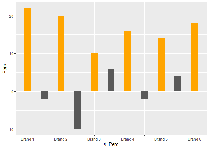
Here is a sketch of getting the two kinds of data into one plot. I invented some data from which to calculate the percentage of each brand.

library(dplyr)
#> 
#> Attaching package: 'dplyr'
#> The following objects are masked from 'package:stats':
#> 
#>     filter, lag
#> The following objects are masked from 'package:base':
#> 
#>     intersect, setdiff, setequal, union
library(ggplot2)
set.seed(1)
BrandData <- sample(c("Brand1","Brand2","Brand3","Brand4","Brand5","Brand6"), 50, replace = TRUE)

DF <- data.frame(Brand= BrandData)
CountDF <- DF %>% group_by(Brand) %>% summarize(Perc = n()/nrow(DF)* 100)
#> `summarise()` ungrouping output (override with `.groups` argument)
CountDF
#> # A tibble: 6 x 2
#>   Brand   Perc
#>   <chr>  <dbl>
#> 1 Brand1   22 
#> 2 Brand2   20 
#> 3 Brand3   10 
#> 4 Brand4   16 
#> 5 Brand5   14.
#> 6 Brand6   18
CountDF <- CountDF %>% mutate(Lag = lag(Perc), Diff = Perc - Lag,
                              X_Perc = 1:6, X_Diff = seq(0.5, 5.5, by = 1))

ggplot(CountDF) + geom_col(aes(X_Perc, Perc), fill = "orange", width = 0.2) +
  geom_col(aes(X_Diff, Diff), width = 0.2) +
  scale_x_continuous(labels = c("Brand 1", "","Brand 2", "","Brand 3", "","Brand 4", "",
                               "Brand 5", "","Brand 6"), breaks = seq(1, 6, by  = 0.5),
                    minor_breaks = NULL)
#> Warning: Removed 1 rows containing missing values (position_stack).

Created on 2021-01-13 by the reprex package (v0.3.0)

Thank you so much @FJCC ! Sounds like this is the solution!
I am a little lost with what is happening here:

mutate(Lag = lag(Perc), Diff = Perc - Lag,
                              X_Perc = 1:6, X_Diff = seq(0.5, 5.5, by = 1))

Can you please explain this one, if you don't mind?
In the meantime, I will try to implement this on my data and hopefully it works for me without any issues.

Thanks again for your help!

I did pack a lot into the mutate() function.
The lag() function take the Perc column and "pushes it down" so that the first row is NA, the second row has the value of the first row of Perc, the third row has the value of the second row of Perc, etc.

The Diff column contains the difference between Perc and Lag. Since Lag contains the Perc value from the previous row, this amounts to the difference between consecutive values of Perc.

The X_Perc and X_Diff columns are just dummy x values for graphing. I could have made them any set of equally spaced values. X_Perc is 1,2,3,4,5,6 and is used for the x values of the Perc data. X_Diff is 0.5, 1.5, 2.5, 3.5, 4.5, 5.5 and is used for the x values of the Diff values. This is what makes the Perc and Diff values appear alternately in the graph. I used the scale_x_continuous in ggplot to replace the labeling of these dummy values with the desired Brand names.

The final data frame looks like this

# A tibble: 6 x 6
  Brand   Perc   Lag   Diff X_Perc X_Diff
  <chr>  <dbl> <dbl>  <dbl>  <int>  <dbl>
1 Brand1   22    NA   NA         1    0.5
2 Brand2   20    22   -2         2    1.5
3 Brand3   10    20  -10         3    2.5
4 Brand4   16    10    6         4    3.5
5 Brand5   14.   16   -2.00      5    4.5
6 Brand6   18    14.   4.00      6    5.5

@FJCC, Thank you so much for explaining this. This definitely is very clear now!

I was trying to implement this into my data. However, I am still running into issues here. I think it would work fine if I had only Brands as one of the variables. However, I have several variables instead which we need for filtering the visualizations. For example, for USA, product GYC, Wave 1, in 2020. So, we do need these extra variables also. I think I am making mistakes with grouping because of several variables.

Data is huge with 12700 rows or so for last 6 years. I have tried to create a reprex for better understanding covering last two years. This is also big for reprex I believe, but I think it covers all the components.

I am still looking to create the chart the way you have created with Brands on X-axis and values as Percentages for Orange bar and Diff for Grey bar.

Do you think this can still work with this kind of data?
Thanks again for your help!

data <- data.frame(
  stringsAsFactors = FALSE,
                      Date = c("2020/01/01 00:00:00","2020/01/01 00:00:00",
                               "2020/01/01 00:00:00","2020/01/01 00:00:00","2020/01/01 00:00:00",
                               "2020/01/01 00:00:00","2020/01/01 00:00:00",
                               "2020/01/01 00:00:00","2020/01/01 00:00:00",
                               "2020/01/01 00:00:00","2020/01/01 00:00:00",
                               "2020/01/01 00:00:00","2020/01/01 00:00:00",
                               "2020/01/01 00:00:00","2020/01/01 00:00:00",
                               "2020/01/01 00:00:00","2020/01/01 00:00:00",
                               "2020/01/01 00:00:00","2020/01/01 00:00:00",
                               "2020/01/01 00:00:00","2020/01/01 00:00:00","2020/01/01 00:00:00",
                               "2020/01/01 00:00:00","2020/01/01 00:00:00",
                               "2019/01/01 00:00:00","2019/01/01 00:00:00",
                               "2019/01/01 00:00:00","2019/01/01 00:00:00",
                               "2019/01/01 00:00:00","2019/01/01 00:00:00",
                               "2019/01/01 00:00:00","2019/01/01 00:00:00",
                               "2019/01/01 00:00:00","2019/01/01 00:00:00",
                               "2019/01/01 00:00:00","2019/01/01 00:00:00",
                               "2019/01/01 00:00:00","2019/01/01 00:00:00","2019/01/01 00:00:00",
                               "2019/01/01 00:00:00","2019/01/01 00:00:00",
                               "2019/01/01 00:00:00","2019/01/01 00:00:00",
                               "2019/01/01 00:00:00","2019/01/01 00:00:00",
                               "2019/01/01 00:00:00","2019/01/01 00:00:00",
                               "2019/01/01 00:00:00","2020/01/01 00:00:00",
                               "2020/01/01 00:00:00","2020/01/01 00:00:00",
                               "2020/01/01 00:00:00","2020/01/01 00:00:00","2020/01/01 00:00:00",
                               "2020/01/01 00:00:00","2020/01/01 00:00:00",
                               "2020/01/01 00:00:00","2020/01/01 00:00:00",
                               "2020/01/01 00:00:00","2020/01/01 00:00:00",
                               "2020/01/01 00:00:00","2020/01/01 00:00:00",
                               "2020/01/01 00:00:00","2020/01/01 00:00:00",
                               "2020/01/01 00:00:00","2020/01/01 00:00:00",
                               "2020/01/01 00:00:00","2020/01/01 00:00:00",
                               "2020/01/01 00:00:00","2020/01/01 00:00:00","2020/01/01 00:00:00",
                               "2020/01/01 00:00:00","2019/01/01 00:00:00",
                               "2019/01/01 00:00:00","2019/01/01 00:00:00",
                               "2019/01/01 00:00:00","2019/01/01 00:00:00",
                               "2019/01/01 00:00:00","2019/01/01 00:00:00",
                               "2019/01/01 00:00:00","2019/01/01 00:00:00",
                               "2019/01/01 00:00:00","2019/01/01 00:00:00",
                               "2019/01/01 00:00:00","2019/01/01 00:00:00",
                               "2019/01/01 00:00:00","2019/01/01 00:00:00","2019/01/01 00:00:00",
                               "2019/01/01 00:00:00","2019/01/01 00:00:00",
                               "2019/01/01 00:00:00","2019/01/01 00:00:00",
                               "2019/01/01 00:00:00","2019/01/01 00:00:00",
                               "2019/01/01 00:00:00","2019/01/01 00:00:00"),
                      Wave = c("Wave 2",
                               "Wave 2","Wave 2","Wave 2","Wave 2","Wave 2",
                               "Wave 2","Wave 2","Wave 2","Wave 2","Wave 2",
                               "Wave 2","Wave 1","Wave 1","Wave 1","Wave 1",
                               "Wave 1","Wave 1","Wave 1","Wave 1","Wave 1",
                               "Wave 1","Wave 1","Wave 1","Wave 2","Wave 2",
                               "Wave 2","Wave 2","Wave 2","Wave 2","Wave 2",
                               "Wave 2","Wave 2","Wave 2","Wave 2","Wave 2",
                               "Wave 1","Wave 1","Wave 1","Wave 1",
                               "Wave 1","Wave 1","Wave 1","Wave 1","Wave 1",
                               "Wave 1","Wave 1","Wave 1","Wave 2","Wave 2",
                               "Wave 2","Wave 2","Wave 2","Wave 2","Wave 2",
                               "Wave 2","Wave 2","Wave 2","Wave 2","Wave 2",
                               "Wave 1","Wave 1","Wave 1","Wave 1","Wave 1",
                               "Wave 1","Wave 1","Wave 1","Wave 1","Wave 1",
                               "Wave 1","Wave 1","Wave 2","Wave 2","Wave 2",
                               "Wave 2","Wave 2","Wave 2","Wave 2","Wave 2",
                               "Wave 2","Wave 2","Wave 2","Wave 2","Wave 1",
                               "Wave 1","Wave 1","Wave 1","Wave 1",
                               "Wave 1","Wave 1","Wave 1","Wave 1","Wave 1",
                               "Wave 1","Wave 1"),
                    Brands = c("Brand 1",
                               "Brand 1","Brand 1","Brand 1","Brand 2","Brand 2",
                               "Brand 2","Brand 2","Brand 3","Brand 3",
                               "Brand 3","Brand 3","Brand 1","Brand 1",
                               "Brand 1","Brand 1","Brand 2","Brand 2","Brand 2",
                               "Brand 2","Brand 3","Brand 3","Brand 3",
                               "Brand 3","Brand 1","Brand 1","Brand 1","Brand 1",
                               "Brand 2","Brand 2","Brand 2","Brand 2",
                               "Brand 3","Brand 3","Brand 3","Brand 3","Brand 1",
                               "Brand 1","Brand 1","Brand 1","Brand 2",
                               "Brand 2","Brand 2","Brand 2","Brand 3","Brand 3",
                               "Brand 3","Brand 3","Brand 1","Brand 1",
                               "Brand 1","Brand 1","Brand 2","Brand 2","Brand 2",
                               "Brand 2","Brand 3","Brand 3","Brand 3",
                               "Brand 3","Brand 1","Brand 1","Brand 1",
                               "Brand 1","Brand 2","Brand 2","Brand 2","Brand 2",
                               "Brand 3","Brand 3","Brand 3","Brand 3",
                               "Brand 1","Brand 1","Brand 1","Brand 1","Brand 2",
                               "Brand 2","Brand 2","Brand 2","Brand 3",
                               "Brand 3","Brand 3","Brand 3","Brand 1","Brand 1",
                               "Brand 1","Brand 1","Brand 2","Brand 2",
                               "Brand 2","Brand 2","Brand 3","Brand 3","Brand 3",
                               "Brand 3"),
                LocationID = c("US1","US1",
                               "US1","US1","US1","US1","US1","US1","US1",
                               "US1","US1","US1","US1","US1","US1","US1",
                               "US1","US1","US1","US1","US1","US1","US1",
                               "US1","US1","US1","US1","US1","US1","US1",
                               "US1","US1","US1","US1","US1","US1","US1",
                               "US1","US1","US1","US1","US1","US1","US1",
                               "US1","US1","US1","US1","CA1","CA1","CA1",
                               "CA1","CA1","CA1","CA1","CA1","CA1","CA1",
                               "CA1","CA1","CA1","CA1","CA1","CA1","CA1",
                               "CA1","CA1","CA1","CA1","CA1","CA1","CA1",
                               "CA1","CA1","CA1","CA1","CA1","CA1","CA1",
                               "CA1","CA1","CA1","CA1","CA1","CA1","CA1",
                               "CA1","CA1","CA1","CA1","CA1","CA1","CA1",
                               "CA1","CA1","CA1"),
                     Tiers = c("Tier 1",
                               "Tier 1","Tier 2","Tier 2","Tier 1","Tier 2",
                               "Tier 1","Tier 2","Tier 1","Tier 1","Tier 2",
                               "Tier 2","Tier 1","Tier 1","Tier 2","Tier 2",
                               "Tier 1","Tier 2","Tier 1","Tier 2","Tier 1",
                               "Tier 1","Tier 2","Tier 2","Tier 1","Tier 1",
                               "Tier 2","Tier 2","Tier 1","Tier 2","Tier 1",
                               "Tier 2","Tier 1","Tier 1","Tier 2","Tier 2",
                               "Tier 1","Tier 1","Tier 2","Tier 2",
                               "Tier 1","Tier 2","Tier 1","Tier 2","Tier 1",
                               "Tier 1","Tier 2","Tier 2","Tier 1","Tier 1",
                               "Tier 2","Tier 2","Tier 1","Tier 1","Tier 2",
                               "Tier 2","Tier 1","Tier 1","Tier 2","Tier 2",
                               "Tier 1","Tier 1","Tier 2","Tier 2","Tier 1",
                               "Tier 1","Tier 2","Tier 2","Tier 1",
                               "Tier 1","Tier 2","Tier 2","Tier 1","Tier 1",
                               "Tier 2","Tier 2"),
                 Product = c("GYC","MCH",
                               "FSN","CPR","GYC","FSN","MCH","CPR","GYC",
                               "MCH","FSN","CPR","GYC","MCH","FSN","CPR",
                               "GYC","FSN","MCH","CPR","GYC","MCH","FSN",
                               "CPR","GYC","MCH","FSN","CPR","GYC","FSN",
                               "MCH","CPR","GYC","MCH","FSN","CPR","GYC",
                               "MCH","FSN","CPR","GYC","FSN","MCH","CPR",
                               "GYC","MCH","FSN","CPR","MCH","GYC","FSN",
                               "CPR","MCH","GYC","FSN","CPR","MCH","GYC",
                               "FSN","CPR","MCH","GYC","FSN","CPR","MCH",
                               "GYC","FSN","CPR","MCH","GYC","FSN","CPR",
                               "MCH","GYC","FSN","CPR","MCH","GYC","FSN",
                               "CPR","MCH","GYC","FSN","CPR","MCH","GYC",
                               "FSN","CPR","MCH","GYC","FSN","CPR","MCH",
                               "GYC","FSN","CPR"),
                    Volume = c(227434228.7,
                               227434228.7,227434228.7,227434228.7,227434228.7,
                               227434228.7,227434228.7,227434228.7,
                               227434228.7,227434228.7,227434228.7,227434228.7,
                               227434228.7,227434228.7,227434228.7,227434228.7,
                               227434228.7,227434228.7,227434228.7,227434228.7,
                               227434228.7,227434228.7,227434228.7,
                               227434228.7,255116000,255116000,255116000,255116000,
                               255116000,255116000,255116000,255116000,
                               255116000,255116000,255116000,255116000,255116000,
                               255116000,255116000,255116000,255116000,
                               255116000,255116000,255116000,255116000,255116000,
                               255116000,255116000,18533000,18533000,
                               18533000,18533000,18533000,18533000,18533000,
                               18533000,18533000,18533000,18533000,18533000,
                               18533000,18533000,18533000,18533000,18533000,
                               18533000,18533000,18533000,18533000,18533000,
                               18533000,18533000,22903662,22903662,22903662,
                               22903662,22903662,22903662,22903662,22903662,
                               22903662,22903662,22903662,22903662,22903662,
                               22903662,22903662,22903662,22903662,22903662,
                               22903662,22903662,22903662,22903662,22903662,
                               22903662),
               WeightedAvg = c(165117250,
                               125316260,111442772.1,47533753.79,219246596.4,
                               216517385.7,212196135.4,145557906.4,173759750.7,
                               172850013.8,149651722.5,82786059.24,
                               143738432.5,131229549.9,105756916.3,45486845.74,
                               214015609.2,212651003.8,211286398.4,139417182.2,
                               178535869.5,167164158.1,152608367.4,79374545.81,
                               173223764,144905888,122455680,44645300,
                               245676708,242870432,241849968,156641224,207154192,
                               195418856,184193752,85208744,169652140,
                               139038220,130874508,44390184,244401128,241594852,
                               238788576,160212848,204603032,196694436,
                               170162372,83933164,12750704,12157648,5671098,
                               1983031,17680482,17550751,16068111,8488114,
                               15178527,13640288,9525962,3817798,11935252,10526744,
                               6115890,1501173,17402487,17254223,15938380,
                               7431733,14233344,12991633,9414764,3354473,
                               15826430.44,13879619.17,7168846.206,2381980.848,
                               21758478.9,21621056.93,20040704.25,
                               9871478.322,18322929.6,16925806.22,11887000.58,
                               4855576.344,15963852.41,13467353.26,7649823.108,
                               2588113.806,22216552.14,22056226.51,20659103.12,
                               9734056.35,18345833.26,17292264.81,11818289.59,
                               4191370.146),
                Percentage = c(0.726,0.551,
                               0.49,0.209,0.964,0.952,0.933,0.64,0.764,
                               0.76,0.658,0.364,0.632,0.577,0.465,0.2,0.941,
                               0.935,0.929,0.613,0.785,0.735,0.671,0.349,
                               0.679,0.568,0.48,0.175,0.963,0.952,0.948,
                               0.614,0.812,0.766,0.722,0.334,0.665,0.545,
                               0.513,0.174,0.958,0.947,0.936,0.628,0.802,
                               0.771,0.667,0.329,0.688,0.656,0.306,0.107,
                               0.954,0.947,0.867,0.458,0.819,0.736,0.514,
                               0.206,0.644,0.568,0.33,0.081,0.939,0.931,
                               0.86,0.401,0.768,0.701,0.508,0.181,0.691,
                               0.606,0.313,0.104,0.95,0.944,0.875,0.431,0.8,
                               0.739,0.519,0.212,0.697,0.588,0.334,0.113,
                               0.97,0.963,0.902,0.425,0.801,0.755,0.516,
                               0.183),
                       Lag = c(NA,0.726,
                               0.551,0.221,NA,0.964,0.952,0.658,NA,0.764,
                               0.76,0.339,0.001,0.632,0.577,0.206,0.029,
                               0.941,0.935,0.648,0.014,0.785,0.735,0.338,
                               0.001,0.679,0.568,0.205,0.035,0.963,0.952,
                               0.652,0.022,0.812,0.766,0.355,NA,0.665,0.545,
                               0.223,0.046,0.958,0.947,0.69,0.016,0.802,
                               0.771,0.335,0.001,0.688,0.356,0.115,0.043,
                               0.954,0.896,0.448,0.026,0.819,0.662,0.207,
                               NA,0.644,0.303,0.114,0.017,0.939,0.877,
                               0.435,0.007,0.768,0.602,0.208,NA,0.691,0.328,
                               0.107,0.016,0.95,0.9,0.457,0.008,0.8,0.65,
                               0.196,NA,0.697,0.341,0.109,0.024,0.97,
                               0.912,0.432,0.009,0.801,0.633,0.229),
                      Diff = c(NA,-0.175,
                               -0.061,-0.012,NA,-0.012,-0.019,-0.018,NA,
                               -0.004,-0.102,0.025,0.631,-0.055,-0.112,-0.006,
                               0.912,-0.006,-0.006,-0.035,0.771,-0.05,
                               -0.064,0.011,0.678,-0.111,-0.088,-0.03,0.928,
                               -0.011,-0.004,-0.038,0.79,-0.046,-0.044,
                               -0.021,NA,-0.12,-0.032,-0.049,0.912,-0.011,
                               -0.011,-0.062,0.786,-0.031,-0.104,-0.006,
                               0.687,-0.032,-0.05,-0.008,0.911,-0.007,-0.029,
                               0.01,0.793,-0.083,-0.148,-0.001,NA,-0.076,
                               0.027,-0.033,0.922,-0.008,-0.017,-0.034,
                               0.761,-0.067,-0.094,-0.027,NA,-0.085,-0.015,
                               -0.003,0.934,-0.006,-0.025,-0.026,0.792,
                               -0.061,-0.131,0.016,NA,-0.109,-0.007,0.004,
                               0.946,-0.007,-0.01,-0.007,0.792,-0.046,-0.117,
                               -0.046)
        )

Here is how I would handle making a graph from your data for a given product , year location and wave. Notice that I calculate Lag and Diff after filtering the data, which I think is the only way to make them meaningful. I could not think of an elegant way to construct a vector of the x axis labels so I just typed them manually.

DataNew <- DATA %>% mutate(Date=ymd_hms(Date),YEAR=year(Date)) %>% 
  filter(YEAR == 2020, Product == "GYC", LocationID == "US1",Wave == "Wave 1") %>% 
  mutate(Lag = lag(Percentage), Diff = Percentage - Lag)

DataNew <- DataNew %>% mutate(X_Perc = seq(1, nrow(DataNew), by=1),
                              X_Diff = seq(0.5,nrow(DataNew)-0.5, by=1))


ggplot(DataNew) + geom_col(aes(X_Perc, Percentage), fill = "orange", width = 0.2) +
  geom_col(aes(X_Diff, Diff), width = 0.2) +
  scale_x_continuous(labels = c("Brand 1", "","Brand 2", "","Brand 3"), 
                     breaks = seq(1, 3, by  = 0.5),
                     minor_breaks = NULL)

Thanks @FJCC!
Actually I am working on a dashboard and so the filtering part will be done using the slicers. I always arrange data with R before going forward. If data can somehow consider right "Diff" considering "Brands" variable, that would work with slicers automatically.

I am not sure if this is possible, though. But thank you so much all the help. I definitely have learnt something new with your help. For this part, I will continue researching.

Thanks again!

This topic was automatically closed 7 days after the last reply. New replies are no longer allowed.

If you have a query related to it or one of the replies, start a new topic and refer back with a link.