Help with species distribution map

I have a data frame which has just three columns: Latitude, Longitude, Species. This df has about 6,000 rows.

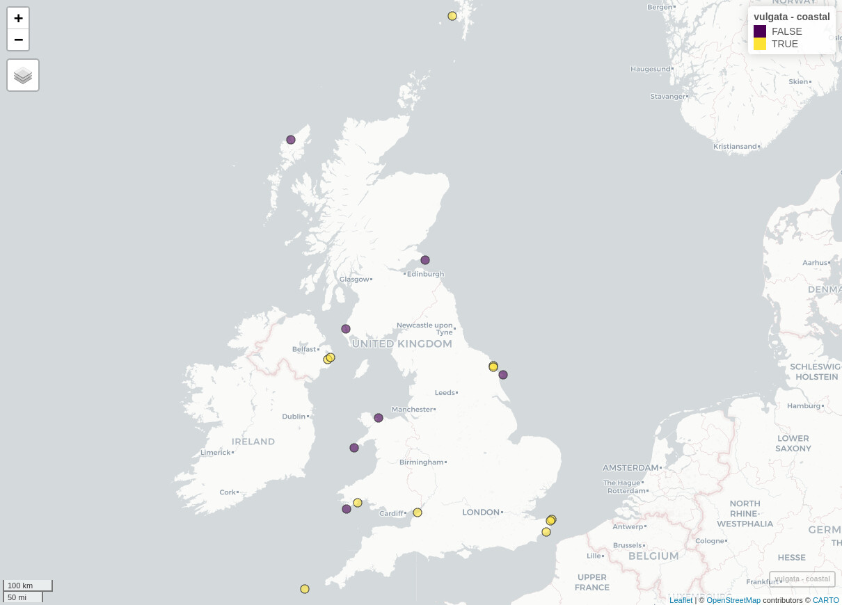
I have successfully mapped it with ggplot, but there are many plot points which are on land and in the middle of the ocean (the species I'm plotting are intertidal - Patella vulgata limpets). I need to get rid of these specific points somehow (one by one from the csv file will not do - this would take days). I only want the high quality plot points which are along the coastline only.

secondly, I need to present the final plot in a 'clean' way so that it can feature in a scientific paper. For this I need to make the plot points appear as a continuous line, or shaded area where the species exists. Right now it looks like a mess because of the number of points.

This is the code I have so far, which does not seem to work. (this was suggested by AI)

########################################################################################

library(sf)
library(ggplot2)

Read the land shapefile into R as an sf object

land_sf <- st_read("ne_50m_land.shp")

Read in the Vulgata.combined data as a data.frame object

Vulgata.combined <- read.csv("Patella GBIF and OBIS COMBINED (new).csv", stringsAsFactors = FALSE)

Use subset function to extract only 'Patella vulgata' rows

Vulgata.combined <- subset(Vulgata.combined, Species == "Patella vulgata")

Remove rows with missing coordinate values

Vulgata.combined <- na.omit(Vulgata.combined[c("Longitude", "Latitude")])

Remove full row duplicates

library(dplyr)
Vulgata.combined <- distinct(Vulgata.combined)

Convert the Vulgata.combined data.frame to an sf object

Vulgata.combined_sf <- st_as_sf(Vulgata.combined, coords = c("Longitude", "Latitude"), crs = 4326)

Perform a spatial join between the Vulgata.combined sf object and the land sf object

Vulgata.land <- st_intersection(Vulgata.combined_sf, land_sf) # this does nothing

#check progress like this
library(sf)
library(ggplot2)
library(progressr)

Remove all points that are more than 100 meters away from land

Vulgata.land <- st_buffer(land_sf, dist = 100) %>%
st_difference(Vulgata.land)

Plot the resulting sf object using ggplot2

ggplot() +
geom_sf(data = land_sf, fill = "lightgray") +
geom_sf(data = Vulgata.land, color = "red", size = 0.5)

here is a snapshot of the df I'm using:

Vulgata.combined
Species Latitude Longitude
1 Patella vulgata 52.75 -4.80
2 Patella vulgata 54.41 -5.63
3 Patella vulgata 51.36 1.44
4 Patella vulgata 54.29 -0.39
5 Patella vulgata 54.96 -5.05
6 Patella vulgata 51.69 -4.69
7 Patella vulgata 60.25 -1.69
8 Patella vulgata 53.32 -4.02
9 Patella vulgata 54.12 -0.08
10 Patella vulgata 58.25 -6.79
11 Patella vulgata 51.49 -2.80
12 Patella vulgata 51.57 -5.03
13 Patella vulgata 51.11 1.28
14 Patella vulgata 54.27 -0.39
15 Patella vulgata 49.96 -6.35
16 Patella vulgata 56.19 -2.55
17 Patella vulgata 51.33 1.41
18 Patella vulgata 54.44 -5.54

Hello, and welcome!

For the first part (filtering your dataset to show only records close to coast) consider this piece of code; what it does is:

  • downloads a shapefile of world coast line; I suggest the one from GISCO (the GIS arm of Eurostat), but there are other options
  • transforms the shapefile from geographical (degrees on a sphere) CRS to planar (meters on a plane) CRS; this greatly speeds up buffering and point - in - polygon operations & pulls out only geometry (without any data)
  • casts the polygon to a line, and buffers it by 5 kilometers - you can vary this, but the idea is to use this to get the tidal area - to filter out finds too far from the coastline either way (inland / seaward)
  • combines the coastal areas to one big bad global multipolygon

The big bad global multipolygon is then used to create a new variable in your vulgata dataset - a logical variable identifying whether the find is plausibly in a tidal area (a Goldilocks - not too far inland, not too far at sea).

I am choosing to plot this goldilocks variable, but you could as easily use ti to filter your observations to keep only the "good ones".

library(sf)
library(dplyr)
library(ggplot2)

vulgata <- tribble(~Species, ~Latitude, ~Longitude,
                  "Patella vulgata", 52.75, -4.80,
                  "Patella vulgata", 54.41, -5.63,
                  "Patella vulgata", 51.36, 1.44,
                  "Patella vulgata", 54.29, -0.39,
                  "Patella vulgata", 54.96, -5.05,
                  "Patella vulgata", 51.69, -4.69,
                  "Patella vulgata", 60.25, -1.69,
                  "Patella vulgata", 53.32, -4.02,
                  "Patella vulgata", 54.12, -0.08,
                  "Patella vulgata", 58.25, -6.79,
                  "Patella vulgata", 51.49, -2.80,
                  "Patella vulgata", 51.57, -5.03,
                  "Patella vulgata", 51.11, 1.28,
                  "Patella vulgata", 54.27, -0.39,
                  "Patella vulgata", 49.96, -6.35,
                  "Patella vulgata", 56.19, -2.55,
                  "Patella vulgata", 51.33, 1.41,
                  "Patella vulgata", 54.44, -5.54) %>% 
  st_as_sf(coords = c("Longitude", "Latitude"), crs = 4326) %>% 
  st_transform(3857)

# get coastal areas as a single multipolygon
coastal_area <- giscoR::gisco_get_coastallines() %>% 
  st_transform(3857) %>% 
  st_geometry()  %>% 
  st_cast("LINESTRING") %>% 
  st_buffer(units::as_units(5, "km")) %>% 
  st_combine()  


# create variable of "coastality" as a logical 
vulgata$coastal <- st_contains(coastal_area,
                               vulgata,
                               sparse = F) %>% 
  .[1,]

# do a visual check
mapview::mapview(vulgata, zcol = "coastal")

As far as the second part (publication quality plots) goes I am afraid that I am not in position to give you a more concrete advice without seeing more of your data.

The best I can do is to point you in the direction of {concaveman} package, which has served me well in plotting concave hulls - your "shaded areas where species exist".

Hi there,

Thanks a million for your help with this!
I've managed to create a csv file with the coastal occurrences of the species only.
Now, I'm having trouble mapping this onto a world map because there are so many individual points. Is it best to plot this data as continuous lines or shaded areas?

Any advice you have is greatly appreciated.

here is a reprex:
Species Latitude Longitude
1 Patella vulgata 6744266 -522088.41
2 Patella vulgata 6439351 -706878.77
3 Patella vulgata 6679876 156960.48
4 Patella vulgata 7369633 -159186.87
5 Patella vulgata 8056069 -567729.40
6 Patella vulgata 8575482 -91281.98
7 Patella vulgata 8184711 -374033.49
8 Patella vulgata 6533322 -390731.41
9 Patella vulgata 6845456 -474221.03
10 Patella vulgata 7198616 -21150.70
11 Patella vulgata 6559615 -163639.65
12 Patella vulgata 7276935 -399636.97

Kind regards,

Bruno

This topic was automatically closed 42 days after the last reply. New replies are no longer allowed.

If you have a query related to it or one of the replies, start a new topic and refer back with a link.