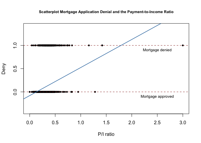
This is a good discussion to continue @startz (my fellow Richard) because I've revisited the linear probability model (PLM). I first saw it a few years ago in an econometric's paper on gender discrimination in the financial industry and was not convinced by the authors' defense of the methodology.
The first example given in the cited text is one in which I had a lot of domain knowledge before 2009, so it serves as a good motivating example. The data to be analyzed concerns mortgage loan application approvals.
---------------------------------------------------------
Describe HMDA (data.frame):

data frame:	2380 obs. of  14 variables
		2380 complete cases (100.0%)

  Nr  ColName    Class    NAs  Levels
  1   deny       factor   .    (2): 1-no, 2-yes
  2   pirat      numeric  .
  3   hirat      numeric  .
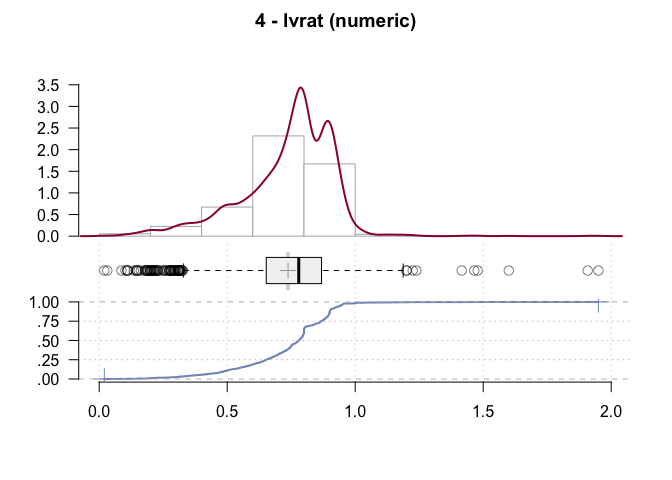
  4   lvrat      numeric  .
  5   chist      factor   .    (6): 1-1, 2-2, 3-3,
                               4-4, 5-5, ...
  6   mhist      factor   .    (4): 1-1, 2-2, 3-3, 4-4
  7   phist      factor   .    (2): 1-no, 2-yes
  8   unemp      numeric  .
  9   selfemp    factor   .    (2): 1-no, 2-yes
  10  insurance  factor   .    (2): 1-no, 2-yes
  11  condomin   factor   .    (2): 1-no, 2-yes
  12  afam       factor   .    (2): 1-no, 2-yes
  13  single     factor   .    (2): 1-no, 2-yes
  14  hschool    factor   .    (2): 1-no, 2-yes
The response (dependent) variable (or regressand) Y is deny, so a value of 0 indicates loan approval (deny is FALSE, 0) while a value of 1 is disapproval.
The treatment (independent) variable (or regressor) X is pirat called P/I ratio, the ratio of scheduled payments of principal and interest on the mortgage loan to income.
The PLM model claims that Y = \beta_0 + \beta_1 * X - u where
\beta_0 is the y-intercept of the regression line
\beta_1 is the slope of the regression line
u is an error term
Earlier in the text, u is explained
the error term u\dots captures additional random effects \dots all the differences between the regression line and the actual observed data. Beside pure randomness, these deviations could also arise from measurement errors or, as will be discussed later, could be the consequence of leaving out other factors that are relevant in explaining the dependent variable.
u, accordingly, may as well stand for Universal Fudge Factor
u is not a term considered necessary in ordinary least square regression, and for good reason. If the question that a linear regression is supposed to answer is what is the probability of observing Y in the presence of X and the answer is 2.54 + 1.39x, plus or minus some other stuff, that is not a very satisfactory state of affairs.
Let's start by ticking off one other consideration. The formula is linear in its parameters, not Y = \beta_0 + \beta_1x^2 + u.
So, here's the example adapted from the text:
library(ggplot2)

data("HMDA",package = "AER")
# inspect the data
DescTools::Desc(HMDA, plotit = TRUE)
#> ------------------------------------------------------------------------------
#> Describe HMDA (data.frame):
#>
#> data frame:  2380 obs. of  14 variables
#>      2380 complete cases (100.0%)
#>
#>   Nr  ColName    Class    NAs  Levels
#>   1   deny       factor   .    (2): 1-no, 2-yes
#>   2   pirat      numeric  .
#>   3   hirat      numeric  .
#>   4   lvrat      numeric  .
#>   5   chist      factor   .    (6): 1-1, 2-2, 3-3, 4-4, 5-5, ...
#>   6   mhist      factor   .    (4): 1-1, 2-2, 3-3, 4-4
#>   7   phist      factor   .    (2): 1-no, 2-yes
#>   8   unemp      numeric  .
#>   9   selfemp    factor   .    (2): 1-no, 2-yes
#>   10  insurance  factor   .    (2): 1-no, 2-yes
#>   11  condomin   factor   .    (2): 1-no, 2-yes
#>   12  afam       factor   .    (2): 1-no, 2-yes
#>   13  single     factor   .    (2): 1-no, 2-yes
#>   14  hschool    factor   .    (2): 1-no, 2-yes
#>
#>
#> ------------------------------------------------------------------------------
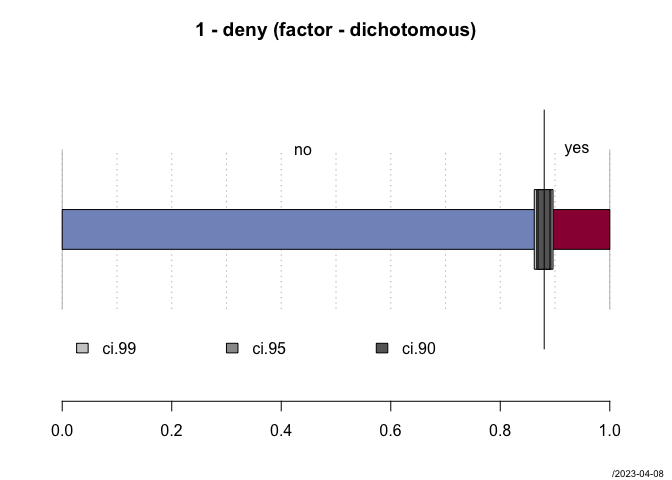
#> 1 - deny (factor - dichotomous)
#>
#>   length      n    NAs unique
#>    2'380  2'380      0      2
#>          100.0%   0.0%
#>
#>       freq   perc  lci.95  uci.95'
#> no   2'095  88.0%   86.7%   89.3%
#> yes    285  12.0%   10.7%   13.3%
#>
#> ' 95%-CI (Wilson)

#> ------------------------------------------------------------------------------
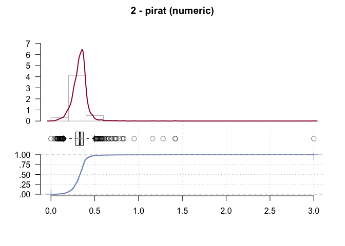
#> 2 - pirat (numeric)
#>
#>   length       n     NAs  unique      0s    mean    meanCI'
#>    2'380   2'380       0     519       1  0.3308    0.3265
#>           100.0%    0.0%            0.0%            0.3351
#>
#>      .05     .10     .25  median     .75     .90       .95
#>   0.1900  0.2300  0.2800  0.3300  0.3700  0.4100    0.4401
#>
#>    range      sd   vcoef     mad     IQR    skew      kurt
#>   3.0000  0.1073  0.3242  0.0608  0.0900  8.0816  174.0668
#>
#> lowest : 0.0, 0.04 (2), 0.056, 0.0699, 0.07 (3)
#> highest: 0.95, 1.16, 1.28, 1.42 (2), 3.0
#>
#> ' 95%-CI (classic)

#> ------------------------------------------------------------------------------
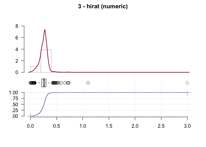
#> 3 - hirat (numeric)
#>
#>     length         n       NAs    unique        0s       mean      meanCI'
#>      2'380     2'380         0       500         3   0.255346    0.251461
#>               100.0%      0.0%                0.1%               0.259231
#>
#>        .05       .10       .25    median       .75        .90         .95
#>   0.120000  0.160000  0.214000  0.260000  0.298825   0.330000    0.350000
#>
#>      range        sd     vcoef       mad       IQR       skew        kurt
#>   3.000000  0.096656  0.378528  0.059304  0.084825  10.306709  277.842289
#>
#> lowest : 0.0 (3), 0.00085, 0.01 (2), 0.02 (3), 0.028
#> highest: 0.72 (2), 0.73, 0.74, 1.1 (2), 3.0
#>
#> heap(?): remarkable frequency (6.0%) for the mode(s) (= 0.28)
#>
#> ' 95%-CI (classic)

#> ------------------------------------------------------------------------------
#> 4 - lvrat (numeric)
#>
#>      length          n        NAs     unique         0s        mean     meanCI'
#>       2'380      2'380          0      1'537          0   0.7377759  0.7305909
#>                 100.0%       0.0%                  0.0%              0.7449609
#>
#>         .05        .10        .25     median        .75         .90        .95
#>   0.3797828  0.4895612  0.6526808  0.7795364  0.8684586   0.9040000  0.9412107
#>
#>       range         sd      vcoef        mad        IQR        skew       kurt
#>   1.9300000  0.1787510  0.2422836  0.1524358  0.2157779  -0.6013342  2.9580578
#>
#> lowest : 0.02, 0.0315107, 0.0869565, 0.1025641, 0.1096491
#> highest: 1.4651163, 1.4782609, 1.6, 1.9083333, 1.95
#>
#> heap(?): remarkable frequency (6.1%) for the mode(s) (= 0.8)
#>
#> ' 95%-CI (classic)

#> ------------------------------------------------------------------------------
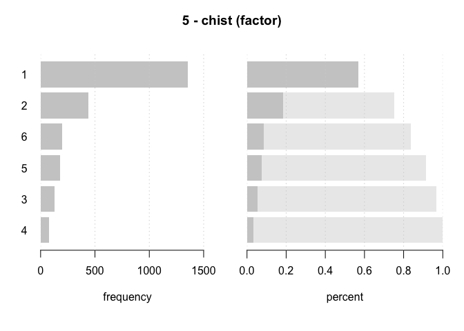
#> 5 - chist (factor)
#>
#>   length      n    NAs unique levels  dupes
#>    2'380  2'380      0      6      6      y
#>          100.0%   0.0%
#>
#>    level   freq   perc  cumfreq  cumperc
#> 1      1  1'353  56.8%    1'353    56.8%
#> 2      2    441  18.5%    1'794    75.4%
#> 3      6    201   8.4%    1'995    83.8%
#> 4      5    182   7.6%    2'177    91.5%
#> 5      3    126   5.3%    2'303    96.8%
#> 6      4     77   3.2%    2'380   100.0%

#> ------------------------------------------------------------------------------
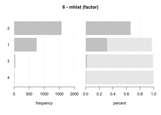
#> 6 - mhist (factor)
#>
#>   length      n    NAs unique levels  dupes
#>    2'380  2'380      0      4      4      y
#>          100.0%   0.0%
#>
#>    level   freq   perc  cumfreq  cumperc
#> 1      2  1'571  66.0%    1'571    66.0%
#> 2      1    747  31.4%    2'318    97.4%
#> 3      3     41   1.7%    2'359    99.1%
#> 4      4     21   0.9%    2'380   100.0%

#> ------------------------------------------------------------------------------
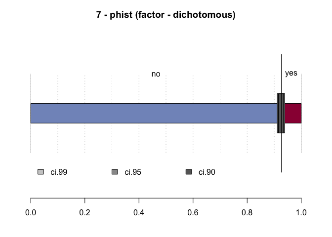
#> 7 - phist (factor - dichotomous)
#>
#>   length      n    NAs unique
#>    2'380  2'380      0      2
#>          100.0%   0.0%
#>
#>       freq   perc  lci.95  uci.95'
#> no   2'205  92.6%   91.5%   93.6%
#> yes    175   7.4%    6.4%    8.5%
#>
#> ' 95%-CI (Wilson)

#> ------------------------------------------------------------------------------
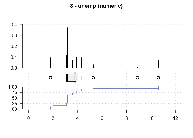
#> 8 - unemp (numeric)
#>
#>   length       n    NAs  unique    0s  mean  meanCI'
#>    2'380   2'380      0      10     0  3.77    3.69
#>           100.0%   0.0%          0.0%          3.86
#>
#>      .05     .10    .25  median   .75   .90     .95
#>     1.80    2.00   3.10    3.20  3.90  5.30   10.60
#>
#>    range      sd  vcoef     mad   IQR  skew    kurt
#>     8.80    2.03   0.54    0.59  0.80  2.53    5.99
#>
#>
#>                value  freq   perc  cumfreq  cumperc
#> 1   1.79999995231628   217   9.1%      217     9.1%
#> 2                  2   148   6.2%      365    15.3%
#> 3   3.09999990463257   275  11.6%      640    26.9%
#> 4   3.20000004768372   877  36.8%    1'517    63.7%
#> 5   3.59999990463257   174   7.3%    1'691    71.1%
#> 6   3.90000009536743   229   9.6%    1'920    80.7%
#> 7   4.30000019073486   220   9.2%    2'140    89.9%
#> 8   5.30000019073486    65   2.7%    2'205    92.6%
#> 9   8.89999961853027    16   0.7%    2'221    93.3%
#> 10  10.6000003814697   159   6.7%    2'380   100.0%
#>
#> ' 95%-CI (classic)

#> ------------------------------------------------------------------------------
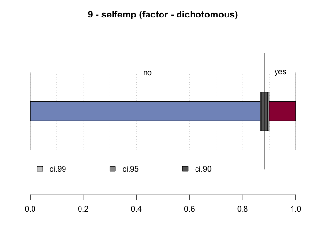
#> 9 - selfemp (factor - dichotomous)
#>
#>   length      n    NAs unique
#>    2'380  2'380      0      2
#>          100.0%   0.0%
#>
#>       freq   perc  lci.95  uci.95'
#> no   2'103  88.4%   87.0%   89.6%
#> yes    277  11.6%   10.4%   13.0%
#>
#> ' 95%-CI (Wilson)

#> ------------------------------------------------------------------------------
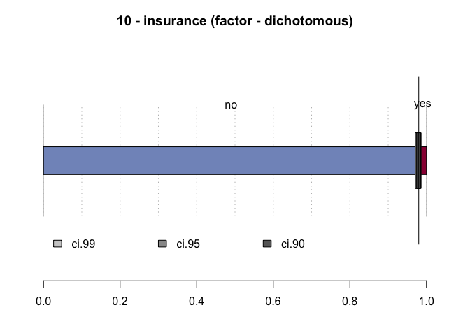
#> 10 - insurance (factor - dichotomous)
#>
#>   length      n    NAs unique
#>    2'380  2'380      0      2
#>          100.0%   0.0%
#>
#>       freq   perc  lci.95  uci.95'
#> no   2'332  98.0%   97.3%   98.5%
#> yes     48   2.0%    1.5%    2.7%
#>
#> ' 95%-CI (Wilson)

#> ------------------------------------------------------------------------------
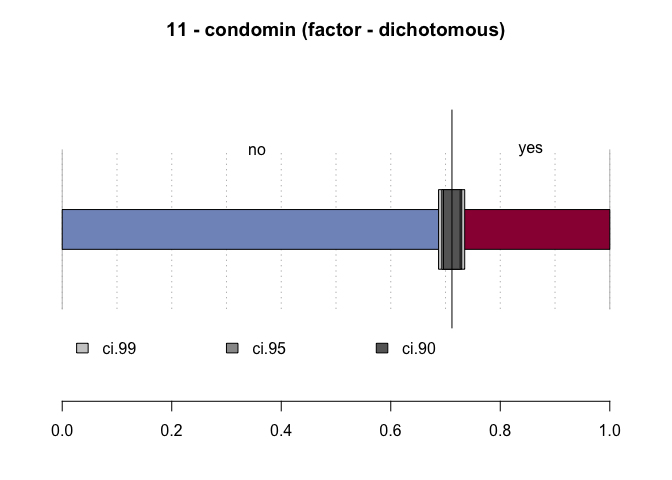
#> 11 - condomin (factor - dichotomous)
#>
#>   length      n    NAs unique
#>    2'380  2'380      0      2
#>          100.0%   0.0%
#>
#>       freq   perc  lci.95  uci.95'
#> no   1'694  71.2%   69.3%   73.0%
#> yes    686  28.8%   27.0%   30.7%
#>
#> ' 95%-CI (Wilson)

#> ------------------------------------------------------------------------------
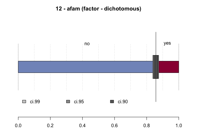
#> 12 - afam (factor - dichotomous)
#>
#>   length      n    NAs unique
#>    2'380  2'380      0      2
#>          100.0%   0.0%
#>
#>       freq   perc  lci.95  uci.95'
#> no   2'041  85.8%   84.3%   87.1%
#> yes    339  14.2%   12.9%   15.7%
#>
#> ' 95%-CI (Wilson)

#> ------------------------------------------------------------------------------
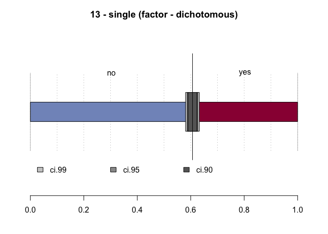
#> 13 - single (factor - dichotomous)
#>
#>   length      n    NAs unique
#>    2'380  2'380      0      2
#>          100.0%   0.0%
#>
#>       freq   perc  lci.95  uci.95'
#> no   1'444  60.7%   58.7%   62.6%
#> yes    936  39.3%   37.4%   41.3%
#>
#> ' 95%-CI (Wilson)

#> ------------------------------------------------------------------------------
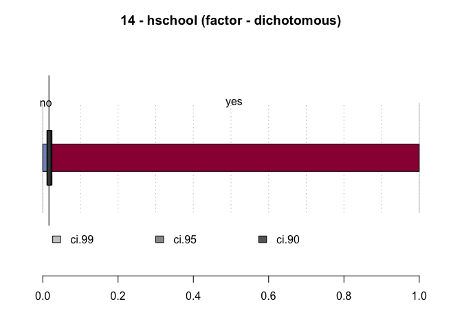
#> 14 - hschool (factor - dichotomous)
#>
#>   length      n    NAs unique
#>    2'380  2'380      0      2
#>          100.0%   0.0%
#>
#>       freq   perc  lci.95  uci.95'
#> no      39   1.6%    1.2%    2.2%
#> yes  2'341  98.4%   97.8%   98.8%
#>
#> ' 95%-CI (Wilson)

# subset the variables to be used in the example
d <- HMDA[1:2]
# convert factor to numeric 1/0
d[,1] <- as.numeric(d[,1]) - 1

# show them
d |> ggplot(aes(pirat,deny)) +
  geom_point() +
  geom_smooth(method = "lm") +
  theme_minimal()
#> `geom_smooth()` using formula = 'y ~ x'

# model

fit <- lm(deny ~ pirat,d)
summary(fit)
#>
#> Call:
#> lm(formula = deny ~ pirat, data = d)
#>
#> Residuals:
#>      Min       1Q   Median       3Q      Max
#> -0.73070 -0.13736 -0.11322 -0.07097  1.05577
#>
#> Coefficients:
#>             Estimate Std. Error t value Pr(>|t|)
#> (Intercept) -0.07991    0.02116  -3.777 0.000163 ***
#> pirat        0.60353    0.06084   9.920  < 2e-16 ***
#> ---
#> Signif. codes:  0 '***' 0.001 '**' 0.01 '*' 0.05 '.' 0.1 ' ' 1
#>
#> Residual standard error: 0.3183 on 2378 degrees of freedom
#> Multiple R-squared:  0.03974,    Adjusted R-squared:  0.03933
#> F-statistic: 98.41 on 1 and 2378 DF,  p-value: < 2.2e-16

# plot from text
plot(x = d$pirat,
     y = d$deny,
     main = "Scatterplot Mortgage Application Denial and the Payment-to-Income Ratio",
     xlab = "P/I ratio",
     ylab = "Deny",
     pch = 20,
     ylim = c(-0.4, 1.4),
     cex.main = 0.8)

# add horizontal dashed lines and text
abline(h = 1, lty = 2, col = "darkred")
abline(h = 0, lty = 2, col = "darkred")
text(2.5, 0.9, cex = 0.8, "Mortgage denied")
text(2.5, -0.1, cex= 0.8, "Mortgage approved")

# add the estimated regression line
abline(fit,
       lwd = 1.8,
       col = "steelblue")

# print robust coefficient summary
coeftest(fit, vcov. = vcovHC, type = "HC1")
#> Error in coeftest(fit, vcov. = vcovHC, type = "HC1"): could not find function "coeftest"

# standard plots (not in text)
par(mfrow = c(2,2))
plot(fit)

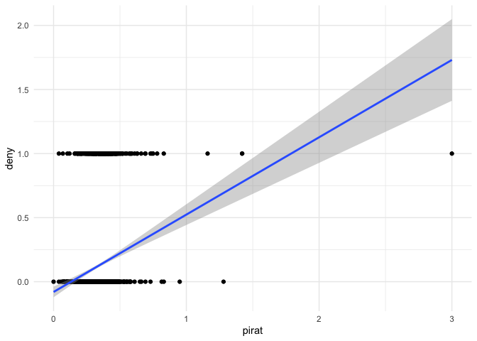
The claim is that the model be interpreted as evidence that each 1% (0.01) increase in the variable pirat increases the probability of denial of a loan application by 0.00604, or 0.6%.
Is that useful information in light of the data? Time for a reality check. There's some bad data
> d[d[2] > 1,]
     deny pirat
621     1  1.16
1095    1  3.00
1321    0  1.28
1928    1  1.42
1929    1  1.42
Even during the height of the mortgage lending craze loans with payment terms amounting to 128% of income were not extended. And, of course the other applications above 100% were rejected. In fact, the "back-end debt-to-income ratio was used and it added to payments of principal and interest credit card, auto loan, student loan and all other disclosed debt. The soft cut-off for that ratio was 38% and of the last 125,000 loan summaries I looked at 55% was the highest I ever saw.
This matters because of the reality distortion field that may be generated. To test, I subset to exclude values greater than 50%. I found that doing so approximately doubled the probability of denial of a loan application for each 1% increase in the P/I ratio. A cautionary tale the moral of which is that while the data may not lie, they are entirely capable of deceit.
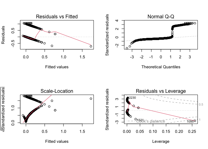
Several points to note on the standard diagnostic plot
- As noted in the text R^2 has no interpretation
- Although linear in the parameters, the residuals vs. fitted plot doesn't cluster around zero
- QQ plot shows residuals are not normally distributed
- Scale-location shows heteroskedascity to the max
- The outliers in residuals vs. leverage probably indicate the influence of the anomolously large values of the variable
pirat
The model also predicts probabilities of denial in excess of 1.
(Left as an exercise—divide the data into training and test sets and compare predictions of the test data to the observed results and compare RMSE to just the proportions in a two-way contingency table.)
The two principal arguments advanced in the case of the linear probability model are simplicity and robustness. We no longer use desk calculators, so the first argument can be dismissed out of hand. Robustness cannot compensate for a non-normal distribution of residuals. Brushed aside is the usually untenable assumption that the u term can be ignored in the calculations and usable results can be obtained by assuming away not only any influence of other variables but their existence also and treating the model as entirely endogenous. As my country cousins say that dog won't hunt.
And that's even before confronting the principal difficulty in the case presented by the OP, which is that not only is the response variable binary, so is the variable being regressed against.
Just. Don't. Go. There.
