Help: Trying to create a column calculation based on a subset of rows in the input table

KathleenC · March 25, 2019, 6:02pm

Hello,
I have a data cleaning task that is unexpectedly throwing me a curveball. I created a small sample set to validate and test against.

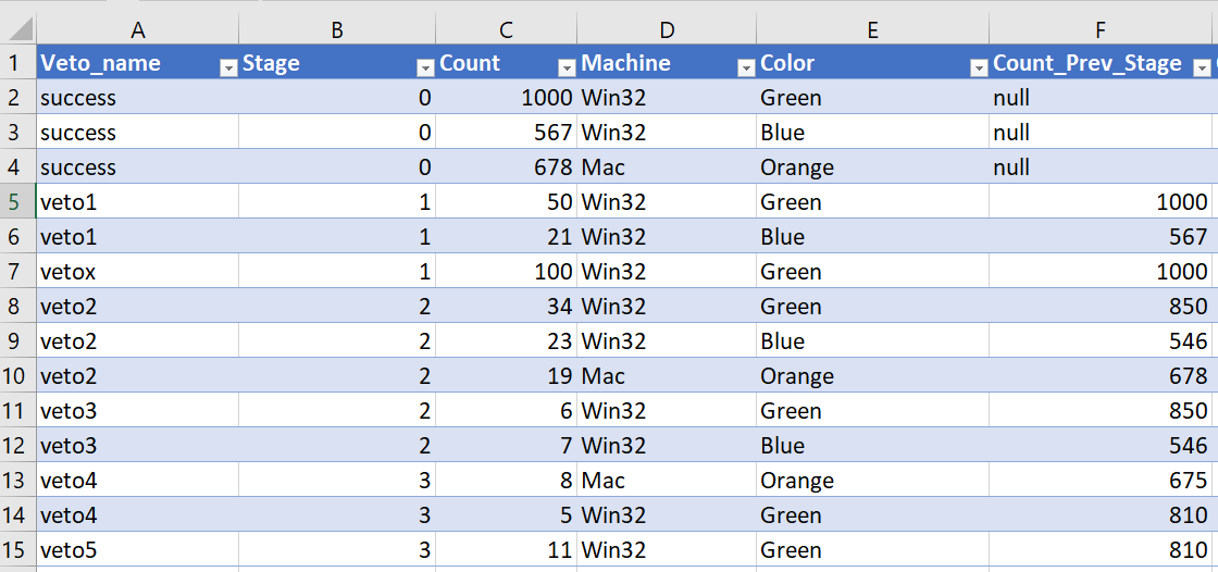
The core of the computation I'm trying to accomplish is to create a new column which contains the count of previous stage (grouped by the metadata). The formula for this is count_at_stage_zero - sum (counts for 0 < stage < current stage).

Stages: 0 is initial so count here is the number of things that began at Stage 0. All other stages the count is really a measure of failure. I view it as "this many things went wrong".

This looks like the following table created in Excel. Count_Prev_Stage is my new column and everything else is my input data.

I don't have code to share since I'm at the "stumped" phase of the process. Any help or direction on how to calculate Count_Prev_Stage would be super appreciated. If there is something I can do to clarify the problem so that help is easier to give please let me know. I'm not sure I've eloquently translated what is in my head to a scoped problem.

Thank you,
Kathleen

andresrcs · March 26, 2019, 12:39am

Hi Kathleen, welcome!
Any chance you could at least share some sample data and a sample output on a copy/paste friendly format?
If you don't know how, here is a blog post by Mara that explains how to do it.

KathleenC · March 26, 2019, 1:11am

Thanks so much @andresrcs! That link was super helpful. I'm hoping I did the reprex correctly.

This is the input dataset:

dataset <- data.frame(stringsAsFactors=FALSE,
   Veto_name = c("success", "success", "success", "veto1", "veto1", "vetox",
                 "veto2", "veto2", "veto2", "veto3", "veto4", "veto4", "veto4",
                 "veto5"),
       Stage = c(0L, 0L, 0L, 1L, 1L, 1L, 2L, 2L, 2L, 2L, 2L, 3L, 3L, 3L),
       Count = c(1000L, 567L, 678L, 50L, 21L, 100L, 34L, 23L, 19L, 6L, 7L, 8L,
                 5L, 11L),
     Machine = c("Win32", "Win32", "Mac", "Win32", "Win33", "Win34", "Win35",
                 "Win36", "Mac", "Win32", "Win32", "Mac", "Win32", "Win32"),
       Color = c("Green", "Blue", "Orange", "Green", "Blue", "Green", "Green",
                 "Blue", "Orange", "Green", "Blue", "Orange", "Green",
                 "Green")
)

This is with the additional column Count_Prev_Stage that I'm trying to calculate (here I just typed in values to the spreadsheet). I'd like to figure out how to calculate this column using R.

result_with_count_prev_stage_col <- data.frame(stringsAsFactors=FALSE,
                                                    Veto_name = c("success", "success", "success", "veto1", "veto1",
                                                                  "vetox",
                                                                  "veto2", "veto2",
                                                                  "veto2",
                                                                  "veto3", "veto4",
                                                                  "veto4", "veto4",
                                                                  "veto5"),
                                                        Stage = c(0L, 0L, 0L, 1L, 1L, 1L, 2L, 2L, 2L, 2L, 2L, 3L, 3L, 3L),
                                                        Count = c(1000L, 567L, 678L, 50L, 21L, 100L, 34L, 23L, 19L, 6L,
                                                                  7L, 8L, 5L,
                                                                  11L),
                                                      Machine = c("Win32", "Win32", "Mac", "Win32", "Win33", "Win34",
                                                                  "Win35",
                                                                  "Win36", "Mac",
                                                                  "Win32", "Win32",
                                                                  "Mac", "Win32",
                                                                  "Win32"),
                                                        Color = c("Green", "Blue", "Orange", "Green", "Blue", "Green",
                                                                  "Green",
                                                                  "Blue", "Orange",
                                                                  "Green", "Blue",
                                                                  "Orange",
                                                                  "Green", "Green"),
                                             Count_Prev_Stage = c("null", "null", "null", "1000", "567", "1000", "850",
                                                                  "546", "678",
                                                                  "850", "546",
                                                                  "675", "810",
                                                                  "810")
                                          )

FJCC · March 26, 2019, 2:33am

Here is an ugly solution that I hope others can improve upon. I get a different answer for the last Mac Orange line, 659. Your table shows 675 but I believe 659 is correct.

library(dplyr)
#> 
#> Attaching package: 'dplyr'
#> The following objects are masked from 'package:stats':
#> 
#>     filter, lag
#> The following objects are masked from 'package:base':
#> 
#>     intersect, setdiff, setequal, union
df <- data.frame(Stage = c(0,0,0,1,1,1,2,2,2,2,2,3,3,3), 
                 Count = c(1000, 567,678,50,21,100,34,23,19,6,7,8,5,11),
                 Machine = c("Win32", "Win32", "Mac", "Win32","Win32","Win32","Win32",
                             "Win32","Mac", "Win32","Win32","Mac","Win32","Win32"),
                 Color = c("Green", "Blue", "Orange", "Green", "Blue", "Green", "Green", 
                           "Blue", "Orange", "Green", "Blue", "Orange", "Green", "Green"))
CumSum = df %>% filter(Stage != 0) %>% group_by(Stage, Machine, Color) %>% 
  mutate(RunSum = cumsum(Count)) %>% ungroup() %>% group_by(Stage, Machine, Color) %>% 
  summarize(StageSum = max(RunSum))
CumSum
#> # A tibble: 7 x 4
#> # Groups:   Stage, Machine [?]
#>   Stage Machine Color  StageSum
#>   <dbl> <fct>   <fct>     <dbl>
#> 1     1 Win32   Blue         21
#> 2     1 Win32   Green       150
#> 3     2 Mac     Orange       19
#> 4     2 Win32   Blue         30
#> 5     2 Win32   Green        40
#> 6     3 Mac     Orange        8
#> 7     3 Win32   Green        16
Total <- CumSum %>% ungroup() %>% group_by(Machine, Color) %>% arrange(Stage) %>% 
  mutate(AllStages = cumsum(StageSum), JoinStage = Stage + 1)
Total
#> # A tibble: 7 x 6
#> # Groups:   Machine, Color [3]
#>   Stage Machine Color  StageSum AllStages JoinStage
#>   <dbl> <fct>   <fct>     <dbl>     <dbl>     <dbl>
#> 1     1 Win32   Blue         21        21         2
#> 2     1 Win32   Green       150       150         2
#> 3     2 Mac     Orange       19        19         3
#> 4     2 Win32   Blue         30        51         3
#> 5     2 Win32   Green        40       190         3
#> 6     3 Mac     Orange        8        27         4
#> 7     3 Win32   Green        16       206         4
df2 <- left_join(df, Total, by = c(Stage = "JoinStage", Machine = "Machine", Color = "Color"))
Orig <- df %>% filter(Stage == 0) %>% select(-Stage)
df2 <- inner_join(df2, Orig, by = c(Machine = "Machine", Color = "Color"), 
                  suffix = c(".df2", ".orig"))
df2 <- df2 %>% mutate(Count_Prev_Stage = ifelse(!is.na(AllStages), Count.orig - AllStages,
                                                Count.orig))
df2 %>% select(Stage, Count.df2, Machine, Color, Count_Prev_Stage)        
#>    Stage Count.df2 Machine  Color Count_Prev_Stage
#> 1      0      1000   Win32  Green             1000
#> 2      0       567   Win32   Blue              567
#> 3      0       678     Mac Orange              678
#> 4      1        50   Win32  Green             1000
#> 5      1        21   Win32   Blue              567
#> 6      1       100   Win32  Green             1000
#> 7      2        34   Win32  Green              850
#> 8      2        23   Win32   Blue              546
#> 9      2        19     Mac Orange              678
#> 10     2         6   Win32  Green              850
#> 11     2         7   Win32   Blue              546
#> 12     3         8     Mac Orange              659
#> 13     3         5   Win32  Green              810
#> 14     3        11   Win32  Green              810

^{Created on 2019-03-25 by the reprex package (v0.2.1)}

andresrcs · March 26, 2019, 2:54am

Another solution but with the same observation about the last Mac Orange line

dataset <- data.frame(stringsAsFactors=FALSE,
                      Veto_name = c("success", "success", "success", "veto1", "veto1", "vetox",
                                    "veto2", "veto2", "veto2", "veto3", "veto4", "veto4", "veto4",
                                    "veto5"),
                      Stage = c(0L, 0L, 0L, 1L, 1L, 1L, 2L, 2L, 2L, 2L, 2L, 3L, 3L, 3L),
                      Count = c(1000L, 567L, 678L, 50L, 21L, 100L, 34L, 23L, 19L, 6L, 7L, 8L,
                                5L, 11L),
                      Machine = c("Win32", "Win32", "Mac", "Win32", "Win32", "Win32", "Win32",
                                  "Win32", "Mac", "Win32", "Win32", "Mac", "Win32", "Win32"),
                      Color = c("Green", "Blue", "Orange", "Green", "Blue", "Green", "Green",
                                "Blue", "Orange", "Green", "Blue", "Orange", "Green",
                                "Green")
)
library(dplyr)
library(tidyr)

dataset %>% 
    mutate(signed_count = if_else(Stage == 0, Count, as.integer(Count * -1))) %>%
    complete(Stage, nesting(Machine, Color)) %>%
    group_by(Machine, Color, Stage) %>%
    summarise(signed_count = sum(signed_count, na.rm = TRUE)) %>%
    arrange(Machine, Color, Stage) %>% 
    mutate(Count_Prev_Stage = cumsum(signed_count), 
           Stage = Stage + 1) %>% 
    right_join(dataset, by = c("Machine", "Color", "Stage")) %>% 
    select(Veto_name, Count, Stage, Machine, Color, Count_Prev_Stage)
#> # A tibble: 14 x 6
#> # Groups:   Machine, Color [3]
#>    Veto_name Count Stage Machine Color  Count_Prev_Stage
#>    <chr>     <int> <dbl> <chr>   <chr>             <int>
#>  1 success    1000     0 Win32   Green                NA
#>  2 success     567     0 Win32   Blue                 NA
#>  3 success     678     0 Mac     Orange               NA
#>  4 veto1        50     1 Win32   Green              1000
#>  5 veto1        21     1 Win32   Blue                567
#>  6 vetox       100     1 Win32   Green              1000
#>  7 veto2        34     2 Win32   Green               850
#>  8 veto2        23     2 Win32   Blue                546
#>  9 veto2        19     2 Mac     Orange              678
#> 10 veto3         6     2 Win32   Green               850
#> 11 veto4         7     2 Win32   Blue                546
#> 12 veto4         8     3 Mac     Orange              659
#> 13 veto4         5     3 Win32   Green               810
#> 14 veto5        11     3 Win32   Green               810

KathleenC · March 26, 2019, 5:56pm

Thanks @FJCC and @andresrcs this is super helpful!

Do you have a recommendation on how to "step through" tidyverse code? I've been reading R4DS and in there the suggestion is to read the pipe as "then". And that kind of helps me understand what is going on, but I find my biggest struggle with the tidyverse is when there are no intermediate variables it's hard for me to intuit what each line is contributing. Perhaps the answer is just more experience...?

FJCC · March 26, 2019, 6:17pm

I too find that long chains of %>% can be confusing. The way I step through the statements is to select part of the code and use CTRL + Enter to execute only the selected portion. Looking at

I might select

CumSum = df %>% filter(Stage != 0)

and look at CumSum to see what happened. Then I would execute

CumSum = df %>% filter(Stage != 0) %>% group_by(Stage, Machine, Color) %>% 
      mutate(RunSum = cumsum(Count))

and look at the new state of CumSum

andresrcs · March 26, 2019, 6:23pm

FJCC advice is a good one, but your phrase is also true, with time and more practice you are just going to start visualing the end result in your head very naturally.

Col · March 27, 2019, 2:03am

Here's one more way.

With pipes, I generally can follow but find it hard sometimes. The person coding typically builds the pipeline together and has the advantage of seeing the intermediate results.

The solution below has a somewhat messy data structure in that I kept all of the columns. To clean it up, the Prev_Stage_Max is equivalent to your Count_Prev_Stage.

dataset <- data.frame(stringsAsFactors=FALSE,
                      Veto_name = c("success", "success", "success", "veto1", "veto1", "vetox",
                                    "veto2", "veto2", "veto2", "veto3", "veto4", "veto4", "veto4",
                                    "veto5"),
                      Stage = c(0L, 0L, 0L, 1L, 1L, 1L, 2L, 2L, 2L, 2L, 2L, 3L, 3L, 3L),
                      Count = c(1000L, 567L, 678L, 50L, 21L, 100L, 34L, 23L, 19L, 6L, 7L, 8L,
                                5L, 11L),
                      Machine = c("Win32", "Win32", "Mac", "Win32", "Win32", "Win32", "Win32",
                                  "Win32", "Mac", "Win32", "Win32", "Mac", "Win32", "Win32"),
                      Color = c("Green", "Blue", "Orange", "Green", "Blue", "Green", "Green",
                                "Blue", "Orange", "Green", "Blue", "Orange", "Green",
                                "Green")
)

library(dplyr)

dataset%>%
  group_by(Machine, Color)%>%
  mutate(Count_0 = max(Count),
         Cum_Continued_Success = Count_0 - (cumsum(Count) - Count_0),
         Prev_Stage = lag(Cum_Continued_Success))%>%
  group_by(Stage, add = TRUE)%>%
  mutate(Prev_Stage_Max = max(Prev_Stage))%>%
  ungroup()

KathleenC · March 27, 2019, 2:15am

Thanks that's a really neat solution. Can you help me understand what the ungroup() at the end is doing? I'm not picking up on a difference (maybe my eyes are missing something), but I'd like to learn what the intended purpose is.

When I run without ungroup()

library(dplyr)
> dataset%>%
+   group_by(Machine, Color)%>%
+   mutate(Count_0 = max(Count),
+          Cum_Continued_Success = Count_0 - (cumsum(Count) - Count_0),
+          Prev_Stage = lag(Cum_Continued_Success))%>%
+   group_by(Stage, add = TRUE)%>%
+   mutate(Prev_Stage_Max = max(Prev_Stage))
# A tibble: 14 x 9
# Groups:   Machine, Color, Stage [10]
   Veto_name Stage Count Machine Color  Count_0 Cum_Continued_Success Prev_Stage Prev_Stage_Max
   <chr>     <int> <int> <chr>   <chr>    <dbl>                 <dbl>      <dbl>          <dbl>
 1 success       0  1000 Win32   Green     1000                  1000         NA             NA
 2 success       0   567 Win32   Blue       567                   567         NA             NA
 3 success       0   678 Mac     Orange     678                   678         NA             NA
 4 veto1         1    50 Win32   Green     1000                   950       1000           1000
 5 veto1         1    21 Win32   Blue       567                   546        567            567
 6 vetox         1   100 Win32   Green     1000                   850        950           1000
 7 veto2         2    34 Win32   Green     1000                   816        850            850
 8 veto2         2    23 Win32   Blue       567                   523        546            546
 9 veto2         2    19 Mac     Orange     678                   659        678            678
10 veto3         2     6 Win32   Green     1000                   810        816            850
11 veto4         2     7 Win32   Blue       567                   516        523            546
12 veto4         3     8 Mac     Orange     678                   651        659            659
13 veto4         3     5 Win32   Green     1000                   805        810            810
14 veto5         3    11 Win32   Green     1000                   794        805            810

When I run with ungroup()

dataset%>%
+   group_by(Machine, Color)%>%
+   mutate(Count_0 = max(Count),
+          Cum_Continued_Success = Count_0 - (cumsum(Count) - Count_0),
+          Prev_Stage = lag(Cum_Continued_Success))%>%
+   group_by(Stage, add = TRUE)%>%
+   mutate(Prev_Stage_Max = max(Prev_Stage))%>%
+   ungroup()
# A tibble: 14 x 9
   Veto_name Stage Count Machine Color  Count_0 Cum_Continued_Success Prev_Stage Prev_Stage_Max
   <chr>     <int> <int> <chr>   <chr>    <dbl>                 <dbl>      <dbl>          <dbl>
 1 success       0  1000 Win32   Green     1000                  1000         NA             NA
 2 success       0   567 Win32   Blue       567                   567         NA             NA
 3 success       0   678 Mac     Orange     678                   678         NA             NA
 4 veto1         1    50 Win32   Green     1000                   950       1000           1000
 5 veto1         1    21 Win32   Blue       567                   546        567            567
 6 vetox         1   100 Win32   Green     1000                   850        950           1000
 7 veto2         2    34 Win32   Green     1000                   816        850            850
 8 veto2         2    23 Win32   Blue       567                   523        546            546
 9 veto2         2    19 Mac     Orange     678                   659        678            678
10 veto3         2     6 Win32   Green     1000                   810        816            850
11 veto4         2     7 Win32   Blue       567                   516        523            546
12 veto4         3     8 Mac     Orange     678                   651        659            659
13 veto4         3     5 Win32   Green     1000                   805        810            810
14 veto5         3    11 Win32   Green     1000                   794        805            810

FJCC · March 27, 2019, 2:49am

ungroup() does not change the data values in any way. It and its partner group_by() add or remove an attribute to the data frame so that other functions, particularly summarize(), will act on sub groups of the data frame. Here is an example showing how the attributes of a data frame change after using group_by() and ungroup(). I do not show the values of the data frame but they are constant throughout the example.

df <- data.frame(Pop = rep(c("a", "b"), 5), Value = seq(1,10))
attributes(df)
#> $names
#> [1] "Pop"   "Value"
#> 
#> $class
#> [1] "data.frame"
#> 
#> $row.names
#>  [1]  1  2  3  4  5  6  7  8  9 10
library(dplyr)

df <- df %>% group_by(Pop)
attributes(df)
#> $names
#> [1] "Pop"   "Value"
#> 
#> $class
#> [1] "grouped_df" "tbl_df"     "tbl"        "data.frame"
#> 
#> $row.names
#>  [1]  1  2  3  4  5  6  7  8  9 10
#> 
#> $groups
#> # A tibble: 2 x 2
#>   Pop   .rows    
#>   <fct> <list>   
#> 1 a     <int [5]>
#> 2 b     <int [5]>
df <- df %>% ungroup()
attributes(df)
#> $names
#> [1] "Pop"   "Value"
#> 
#> $class
#> [1] "tbl_df"     "tbl"        "data.frame"
#> 
#> $row.names
#>  [1]  1  2  3  4  5  6  7  8  9 10

^{Created on 2019-03-26 by the reprex package (v0.2.1)}
It is a good idea to use ungroup() at the end of a chain of commands so you do not get surprised if you use the data frame later in your code, forgetting about the grouping.

Col · March 27, 2019, 11:09am

The one without the ungroup() has an extra line under a Tibble 14 x 9. The extra line indicates that there are groups.

Groups are fine but easy to forget. I always ungroup() to prevent a mistake down the road where I don't want a summary statistic by a group.

kenbutler · March 29, 2019, 3:56pm

I tell my students "run it one line at a time". I do this by moving the pipe symbol at the end of a line down to the next line (by moving to before it and pressing enter), and then running the pipe from its start to where it now ends, and having "nothing" on the end of the line will display what you have so far. (If you run the whole chunk you'll get an error about the line with the pipe symbol that is now on the front, but don't worry about that.)

system · April 5, 2019, 3:57pm

This topic was automatically closed 7 days after the last reply. New replies are no longer allowed.

If you have a query related to it or one of the replies, start a new topic and refer back with a link.