Help in determining whether a sample is representative

[aarontimo]

Hi there,

I was wondering if there is a way to test in RStudio whether survey results are representative of a population?

My colleagues and I ran a survey that was open to members of a profession in a specific jurisdiction (i.e. self-selecting survey). We received almost 400 responses. I have demographic data for the entire population (n=17000) in the same jurisdiction (i.e. gender, age, location). These demographics are relevant to our study.

I was thinking of producing a histogram with, for example, the percentage of males, females and non-binary from the survey and either using a facet or otherwise adding the percentage gender spilt to the histogram. And doing the same for the other relevant demographic variables. However, this feels a little unscientific - i.e. just visualising comparing the distribution of the datasets.

Do I need to calculate/use SE (standard error)? Is there some other way to determine whether the responses received in a self-selecting survey are representative of the total population?

Any advice or recommendations would be gratefully appreciated.

[technocrat]

Representative is a judgment call. The tools to aid in forming the judgment vary by domain and the nature of the data. I'd suggest approaching it from a functional analytic framework. f(x) = y. where x is the object to hand, y is the object desired and f is the function to apply to x to return y.

In this case you have two tables, one with n = 400, representing the demographic variables collected on the responding subjects and another with n = 17000 with the same variables for the population of interest. By design, the first is a subset of the second. By what measure(s) do the two tables differ apart from n?

If you have the 17,000 records, and not just their summary statistics, measures of central tendency can be compared and an assessment as to whether the population and subset have means that differ to a greater tolerance than would be expected solely as a result of random variation. A similar estimate can be made for differences in the median. Distribution differences can be considered.

One way to do those three assessments for a variable age, for example would a notched boxplot to provide a visual comparison of mean, median and the prevalence of outliers. That may be sufficient clearly to show that while the population has a mean age of 50, a median age of 37, and few instances of representatives above and below 1.5 times the difference between the 25th and 75th percentile (the interquartile distance), the surveyed population has a mean of 30, a median of 27 and noticeable presence of outliers in the upper range. It would be possible to put a finer gloss on that, but its a clear difference that stands out clearly. On the other hand, if they look closer, there are tests to put a number on it.

Beginning with the variables that, in your assessment, are most relevant to the survey responses, an exploratory data analysis with boxplots for the continuous variables would be a good place to start.

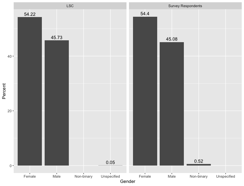
On the other hand, for categorical and ordinal variables, different tools are needed. Contingency tables are helpful. For example,

library(vcd)
#> Loading required package: grid
HairEyeColor
#> , , Sex = Male
#> 
#>        Eye
#> Hair    Brown Blue Hazel Green
#>   Black    32   11    10     3
#>   Brown    53   50    25    15
#>   Red      10   10     7     7
#>   Blond     3   30     5     8
#> 
#> , , Sex = Female
#> 
#>        Eye
#> Hair    Brown Blue Hazel Green
#>   Black    36    9     5     2
#>   Brown    66   34    29    14
#>   Red      16    7     7     7
#>   Blond     4   64     5     8
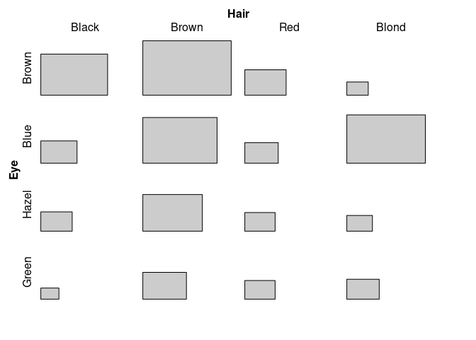
(hec <- margin.table(HairEyeColor, 2:1))
#>        Hair
#> Eye     Black Brown Red Blond
#>   Brown    68   119  26     7
#>   Blue     20    84  17    94
#>   Hazel    15    54  14    10
#>   Green     5    29  14    16
tile(hec)

^{Created on 2022-11-11 by the reprex package (v2.0.1)}

Finally, you could compare the n = 400 with repeated random samples of the same size from the n = 17000 in terms of how different or not the observed demographics are to what would have been obtained by random sampling.

[aarontimo]

Thank you @technocrat. Your explanation is very helpful. Explains why I couldn't find a straightforward answer...there really isn't one.

Unfortunately, for variables of age and gender I only have summary data for the population. Would something like this suffice

Or is there something more scientific I should consider for these variables where only summary data is available?

I'd never seen a margin.table before and that will be really useful of comparing location.

[technocrat]

It's not science so much as conveying the data you have, both from the respondents and the population, in a way that is both accurate and fairly supports the inferences that you are suggesting be drawn. Here, I would say something along the lines of

The reported genders of the respondents and the population at large are comparable for female and male categories. The non-binary and unspecified categories of the two groups differ, but the categories represent quite small portions of each group.

You might want to note that the LSC non-binary category rounded down to zero, if that is true. Otherwise, it appears that the respondents group, which is non-zero, could not be a subset of LSC.

I'd be inclined for data this similar to present the comparison in tabular form unless companion demographics show more variability. I'd do them all as tables or charts, not mixed, though.

Avoiding "representative" as a description fairly relieves you of the burden of searching for some metric to put a hue on the question how representative. The numbers are simple, your presentation discloses it is a sample of convenience of self-selected respondents and for this demographic, at least, the reader would have everything necessary to form her judgment as to comparability.

[aarontimo]

Thank you @technocrat. Again, this useful advice. I think we will try to avoid claims that our dataset is representative but leave it to the reader to make their own call on whether our recommendations are applicable to the population.

Thank you again!