Heatmap using tigris & zcats - mapping zipcodes

[technobrat]

Hi,

I am trying to create a Heatmap of perc_tech_jobs for different zipcodes, which I believe are from the Los Angeles area. I couldn't find this kind of map based off zipcodes and the closest I was able to find was from this source: zcta

I read about zctas and for what I understood if I provide the first two digits of the zipcode the zctas() function would return the polygons for the respective codes. I am unfamiliar with plotting maps and I kind of got the parts I want to some extent but I'm not quite sure how to tie everything together.

I believe that I need to overlay the two maps, remove all these coordinates and then have a color gradient, possibly interactive map where I get the fill gradient and the choice to hover the mouse over the map to see what the actual value is.

library(tidyverse)
library(sf)
#> Linking to GEOS 3.9.1, GDAL 3.2.1, PROJ 7.2.1
library(tigris)
#> To enable 
#> caching of data, set `options(tigris_use_cache = TRUE)` in your R script or .Rprofile.


# Sample df
plot_ready <- tibble(
  zip_code = seq(90001,90015,1),
  tot_employment = c(8538,3175,7066,9795,5932,8799,13410,4823,8,25845,8423,145589,16171,11389,25922),
  tot_tech = c(192,8,43,824,520,384,386,90,0,5449,92,2843,3536,2041,1923),
  perc_tech_jobs = c("2.25%","0.25%","0.61%","8.41%","8.77%","4.36%","2.88%","1.87%","0.00%"  ,"21.08%","1.09%","1.95%", 
                     "21.87%","17.92%","7.42%")
)

# zcta is based on the first 2 zipcode digits 
zip_to_zcta <- plot_ready$zip_code %/% 1000

# polygons from zctas
poly_zctas <- zctas(cb = TRUE, starts_with = zip_to_zcta)
#> ZCTAs can take several minutes to download.  To cache the data and avoid re-downloading in future R sessions, set `options(tigris_use_cache = TRUE)`


# Specifying LA urban areas.
uas <- urban_areas() %>% filter(str_detect(NAME10,"Los Angeles"))

# plotting desired zipcodes
ggplot(poly_zctas, fill = plot_ready$perc_tech_jobs) +
  geom_sf()

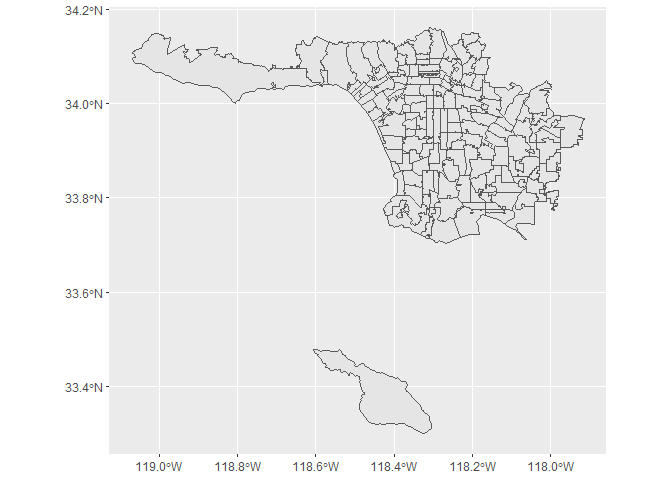
# Missing parts of the map? 
ggplot(uas) + 
  geom_sf()

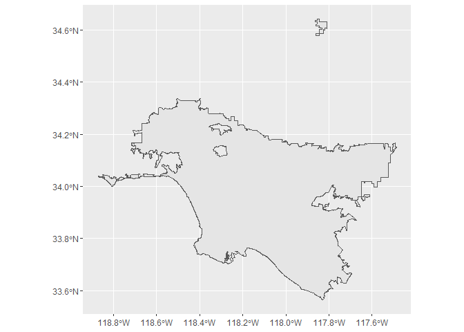
^{Created on 2021-09-29 by the reprex package (v2.0.1)}

I'm uncertain on how to handle these polygons to give me the map I'm trying to achieve. Not sure as well if the sf() package is the one that should handle the fill for the heatmap and how to go about it.

I believe using leaflet() could also be another option, not sure if it would make plotting process any easier.

Thank you for your input and time.

[jrmuirhead]

HI @technobrat ,
You were on the right track. I made a couple of changes to your code including setting the data type of perc_tech_jobs to numeric in order to create a color gradient instead of separate categories, and converting the column zip_code to character in order to join the table plot_ready to poly_zctas.

library(tidyverse)
library(sf)
#> Linking to GEOS 3.9.1, GDAL 3.3.2, PROJ 8.1.1
#> Linking to GEOS 3.9.1, GDAL 3.2.1, PROJ 7.2.1
library(tigris)
#> To enable 
#> caching of data, set `options(tigris_use_cache = TRUE)` in your R script or .Rprofile.
options(tigris_use_cache = TRUE)


# Sample df. Changed perc_tech_jobs to numeric for
# creating gradient instead of categories

plot_ready <- tibble(
  zip_code = seq(90001, 90015, 1),
  tot_employment = c(8538, 3175, 7066, 9795, 5932, 8799, 13410, 4823, 8, 25845,
    8423, 145589, 16171, 11389, 25922),
  tot_tech = c(192, 8, 43, 824, 520, 384, 386, 90, 0, 5449, 92, 2843, 3536,
    2041, 1923),
  perc_tech_jobs = c(2.25, 0.25, 0.61, 8.41, 8.77, 4.36, 2.88, 1.87, 0.00,
    21.08, 1.09, 1.95, 21.87, 17.92, 7.42)) %>%
mutate(zip_to_zcta = zip_code %/% 1000)

# zcta is based on the first 2 zipcode digits

zip_to_zcta <- plot_ready$zip_code %/% 1000

# Convert zip code to character for joining with poly_zctas
plot_ready <- plot_ready %>%
  mutate(zip_code = as.character(zip_code))


# polygons from zctas
poly_zctas <- zctas(cb = TRUE, starts_with = zip_to_zcta) %>%
  left_join(plot_ready, by = c("ZCTA5CE10" = "zip_code"))


# Specifying LA urban areas.
uas <- urban_areas() %>% filter(str_detect(NAME10, "Los Angeles"))

# For plotting with data from 2 sources, leave the arguments to ggplot
# blank and supply the data argument to each of the geoms.

ggplot() +
  geom_sf(data = uas) +
  geom_sf(data = poly_zctas, aes(fill = perc_tech_jobs))

^{Created on 2021-09-29 by the reprex package (v2.0.1)}**

[technobrat]

@jrmuirhead thank you for your assistance.

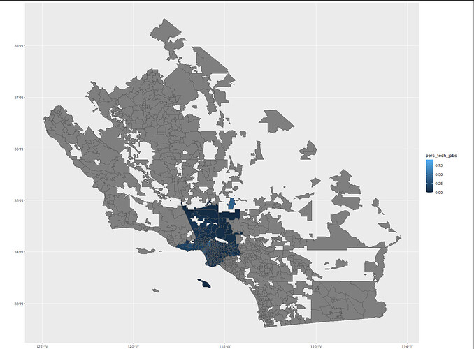
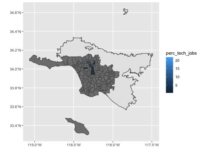
I was able to make the following plot:

A few questions, I believe the zip codes I have are also outside of what is considered uas - Urban Areas from LA.

• How do I change the outline color of that polygon for example so it stands out - therefore ensuring it was plotted.
• How do I drop these "irrelevant"/ grey zip code areas from the map to reduce clutter.
• How do I centralize the map?
• Don't need lat/ long axis, how would we remove them?

[jrmuirhead]

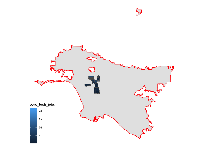
Hi @technobrat,

@technobrat

Q1. - How do I change the outline color of that polygon for example so it stands out - therefore ensuring it was plotted.
A1 - I'm not sure which polygon you need outlined, but geom_sf follows the same rules as other geoms in ggplot2, with color = for outlines, and fill = for fills. See how I specified the red outline color for the uas simple feature in the call to ggplot.

Q2 - How do I drop these "irrelevant"/ grey zip code areas from the map to reduce clutter.
A2 - You can use the same dplyr actions on a simple features object to filter out rows, or add columns, joins, etc. In this example, I filtered out all rows of poly_zctas where perc_tech_jobs data was missing.

Q3 - How do I centralize the map?
A3 - I'm not sure what you mean by this, as a lot of the marginal space is dictated by the coordinate system and the data you have. In this case, the default is using a datum of EPSG:4326, which is the default for longitude, latitude.

Q4 - Don't need lat/ long axis, how would we remove them?
A4 - I've added theme_map() from ggthemes as a quick way to remove axis ticks and labels.

library("tidyverse")
library("sf")
#> Linking to GEOS 3.9.1, GDAL 3.3.2, PROJ 8.1.1
library("ggthemes")
library("tigris")

options(tigris_use_cache = TRUE)


# Sample df. Changed perc_tech_jobs to numeric for
# creating gradient instead of categories

plot_ready <- tibble(
  zip_code = seq(90001, 90015, 1),
  tot_employment = c(8538, 3175, 7066, 9795, 5932, 8799, 13410, 4823, 8, 25845,
    8423, 145589, 16171, 11389, 25922),
  tot_tech = c(192, 8, 43, 824, 520, 384, 386, 90, 0, 5449, 92, 2843, 3536,
    2041, 1923),
  perc_tech_jobs = c(2.25, 0.25, 0.61, 8.41, 8.77, 4.36, 2.88, 1.87, 0.00,
    21.08, 1.09, 1.95, 21.87, 17.92, 7.42)) %>%
mutate(zip_to_zcta = zip_code %/% 1000)

# zcta is based on the first 2 zipcode digits

zip_to_zcta <- plot_ready$zip_code %/% 1000

# Convert zip code to character for joining with poly_zctas
plot_ready <- plot_ready %>%
  mutate(zip_code = as.character(zip_code))


# polygons from zctas
poly_zctas <- zctas(cb = TRUE, starts_with = zip_to_zcta) %>%
  left_join(plot_ready, by = c("ZCTA5CE10" = "zip_code")) %>%
  filter(!is.na(perc_tech_jobs))


# Specifying LA urban areas.
uas <- urban_areas() %>% filter(str_detect(NAME10, "Los Angeles"))

# For plotting with data from 2 sources, leave the arguments to ggplot
# blank and supply the data argument to each of the geoms.

ggplot() +
  geom_sf(data = uas, color = "red") +
  geom_sf(data = poly_zctas, aes(fill = perc_tech_jobs)) +
  theme_map()

^{Created on 2021-09-30 by the reprex package (v2.0.1)}

[technobrat]

@jrmuirhead Thank you for the pristine and clear assistance! This was amazing thank you, I believe that these examples and reprex are a great point for people attempting the same.

Much appreciated.