Heatmap from image background

[yui_2000]

I’d like to create a plot that visualizes the number of defects at specific positions on this image.
The defect data will come from a CSV file, and the goal is to highlight areas on the image using a color gradient—from high to low defect frequency. For example, something like this:

However, I’m not sure how to approach this problem.
Any guidance or suggestions would be greatly appreciated!

Thank you in advance.

[FJCC]

Here is a simple example of how to do a schematic representation of the layout while coloring the shapes according to the defects. Making an exact replica of the drawing with ggplot would be very tedious, unless there is a package for that I'm unaware of.

library(ggplot2)

DF <- data.frame(Centers_x = c(1, 1, 3, 3, 5, 5, 7, 7),
                 Centers_y = c(3.5, 6.5, 2, 5, 3.5, 6.5, 2, 5),
                 Width = rep(0.75, 8), Height = rep(2, 8),
                 Defects = c(0, 1, 0, 0, 3, 0, 2, 1))
ggplot(DF, aes(x = Centers_x, y = Centers_y, width = Width, height = Height, fill = Defects)) + geom_tile() +
  geom_text(aes(label = Defects), color = "white")

^{Created on 2025-08-25 with reprex v2.1.1}

[margusl]

What kind of position data do you have? Component or nest IDs, coordinates, ... ?

Anyway, if you can get that image in a vector form that's supported by Vector drivers — GDAL documentation, your targets being polygons, you could handle this as a spatial task and create a Choropleth map | the R Graph Gallery

Assuming you are working in manufacturing, you can probably find someone in your organization who can provide you a DXF-file of that carrier.

Though you could trace / vectorize that raster image yourself or just redraw it in CAD or vector program of choice.

---

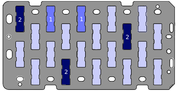
Here's an example with a super-crude & semi-automatic trace from Inkscape, saved as DXF:

library(sf)
#> Linking to GEOS 3.13.1, GDAL 3.11.0, PROJ 9.6.0; sf_use_s2() is TRUE
library(dplyr, warn.conflicts = FALSE)
library(ggplot2)

dxf <- "https://gist.githubusercontent.com/marguslt/fdb11f9558fd592cc150083b31d6e1e4/raw/c91f16041323a575852bc94f43546fa33c780fea/carrier.dxf"
carrier_sf <- 
  # read shapes from DXF,
  # guide GDAL DXF driver to return polygons instead of lines
  read_sf(dxf, options = "CLOSED_LINE_AS_POLYGON=YES") |> 
  select(geometry) 

# detect nest polygons by area, arrange by centroid coordinates & assign IDs 
is_nest <- between(st_area(carrier_sf$geometry), 100, 200)
nests_sf <- 
  carrier_sf[is_nest,] |> 
  mutate(cntr = st_centroid(geometry) |> st_coordinates()) |> 
  arrange(cut(cntr[,2] , breaks = 4) |> desc(), cntr[,1]) |> 
  tibble::rowid_to_column("nest") |> 
  select(-cntr)
print(nests_sf, n = 5)
#> Simple feature collection with 20 features and 1 field
#> Geometry type: POLYGON
#> Dimension:     XY
#> Bounding box:  xmin: 12.2115 ymin: 4.597116 xmax: 147.6006 ymax: 77.62202
#> CRS:           NA
#> # A tibble: 20 × 2
#>    nest                                                                 geometry
#>   <int>                                                                <POLYGON>
#> 1     1 ((19.527 54.69592, 19.5435 57.14332, 19.3856 59.13972, 19.2282 61.13612…
#> 2     2 ((47.8992 54.37602, 48.2222 56.80602, 47.8282 59.23342, 47.4361 61.2788…
#> 3     3 ((76.4706 56.77042, 76.2716 59.35012, 75.9996 61.39162, 76.2616 63.4512…
#> 4     4 ((104.9456 56.68702, 104.7476 59.26672, 104.4756 61.17532, 104.7376 63.…
#> 5     5 ((133.5776 56.59252, 133.5546 58.03192, 133.1806 59.36232, 132.7836 61.…
#> # ℹ 15 more rows

# detect outline polygon by area, subtract other polygons to create holes
outline_idx <- st_area(carrier_sf) |> which.max()
outline_sf <- st_difference(carrier_sf[outline_idx,], st_union(carrier_sf[-outline_idx,]))
outline_sf
#> Simple feature collection with 1 feature and 0 fields
#> Geometry type: POLYGON
#> Dimension:     XY
#> Bounding box:  xmin: 0 ymin: 1.6e-05 xmax: 160.0676 ymax: 82.28542
#> CRS:           NA
#> # A tibble: 1 × 1
#>                                                                         geometry
#> *                                                                      <POLYGON>
#> 1 ((1.2509 2.243116, 0.2348 4.497916, 0.132 7.066116, 0.0933 9.637116, 0.0675 1…

plot(outline_sf)

# some defects
defects <- 
  tribble(
    ~nest, ~n_defects,
    1,     2,
    2,     1,
    3,     1,
    9,     2,
   17,     2)

# join defects to nests sf object
with_defects_sf <- left_join(nests_sf, defects, by = "nest")
print(with_defects_sf, n = 10)
#> Simple feature collection with 20 features and 2 fields
#> Geometry type: POLYGON
#> Dimension:     XY
#> Bounding box:  xmin: 12.2115 ymin: 4.597116 xmax: 147.6006 ymax: 77.62202
#> CRS:           NA
#> # A tibble: 20 × 3
#>     nest                                                      geometry n_defects
#>    <dbl>                                                     <POLYGON>     <dbl>
#>  1     1 ((19.527 54.69592, 19.5435 57.14332, 19.3856 59.13972, 19.22…         2
#>  2     2 ((47.8992 54.37602, 48.2222 56.80602, 47.8282 59.23342, 47.4…         1
#>  3     3 ((76.4706 56.77042, 76.2716 59.35012, 75.9996 61.39162, 76.2…         1
#>  4     4 ((104.9456 56.68702, 104.7476 59.26672, 104.4756 61.17532, 1…        NA
#>  5     5 ((133.5776 56.59252, 133.5546 58.03192, 133.1806 59.36232, 1…        NA
#>  6     6 ((33.7772 37.88832, 34.0926 40.30972, 33.8301 42.73022, 33.5…        NA
#>  7     7 ((62.0827 37.93202, 62.4143 40.40492, 62.1196 42.86252, 61.9…        NA
#>  8     8 ((90.6496 38.16172, 90.9966 40.51642, 90.5836 42.86252, 90.1…        NA
#>  9     9 ((119.1716 40.28812, 118.9736 42.86782, 118.7016 44.77642, 1…         2
#> 10    10 ((147.4146 40.34892, 147.3336 42.44872, 147.1926 44.54522, 1…        NA
#> # ℹ 10 more rows

# plot
with_defects_sf |> 
  ggplot() +
  # outline layer
  geom_sf(data = outline_sf) +
  # nests layer
  geom_sf(aes(fill = n_defects), show.legend = FALSE) +
  # labels
  geom_sf_label(aes(label = n_defects), alpha = .7) +
  scale_fill_fermenter(palette =  "OrRd", direction = 1, na.value = "gray95") +
  theme_minimal() +
  theme(axis.title = element_blank(), axis.text = element_blank(), panel.grid = element_blank())
#> Warning: Removed 15 rows containing missing values or values outside the scale range
#> (`geom_label()`).

[yui_2000]

Yeah, I think that what I need.
Thank you very much