p <- ggplot(df.reduce, aes(x = UNIQUE_CARRIER, y = GROUND_TIME, weight = DEPARTURES_PERFORMED)) +
geom_boxplot()
p + theme(axis.text.x = element_text(angle = 90, vjust = 0.5)) + ylim(0, 60)
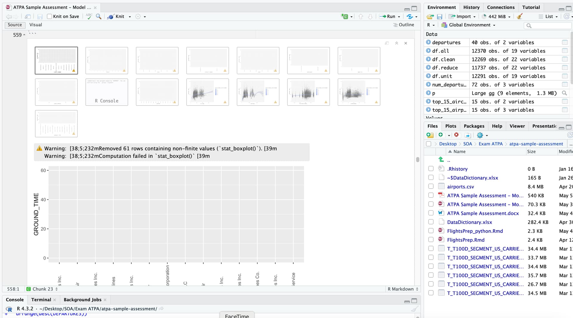
most of the graphs cannot be shown correctly and there're some error msg like "Warning: e[38;5;232mRemoved 61 rows containing non-finite values (stat_boxplot() ).e[39m Warning: e[38;5;232mComputation failed in stat_boxplot() e[39m”
Thanks for providing code. Could you kindly take further steps to make it easier for other forum users to help you? Share some representative data that will enable your code to run and show the problematic behaviour.
How do I share data for a reprex?
You might use tools such as the library datapasta, or the base function dput() to share a portion of data in code form, i.e. that can be copied from forum and pasted to R session.
When I run chunk 1 all the way to chunk 23 inside the file "ATPA Sample Assessment - Model Solution.Rmd”
the above problem occurs with the above error messages
It is big messy .rmd but I think I have hacked my way through it and I cannot reproduce the problem. I don't think you need worry about the Warnings. This just means that some rows in your data set have some missing data points. This is pretty normal in a data set like the one you are using.
When I run the original .rmd, it is fine long past chunk 23.
Does the code below work for you? I just stripped out all the text and redundant data check and ran the working code as a regular script.
I am afraid I don't know what to suggest at the moment.
library(dplyr)

# Use function to do initial editing on each file as it is read in to save memory
read_boise <- function(file) {
  df.all_cities <- read.csv(file, stringsAsFactors = TRUE)
  df.boise <- df.all_cities %>%
              filter(ORIGIN == "BOI" | DEST == "BOI") %>% # BOI is Boise per data dictionary
              mutate(YEAR = as.factor(YEAR),
                     QUARTER = as.factor(QUARTER),
                     MONTH = as.factor(MONTH),
                     AIRCRAFT_TYPE = as.factor(AIRCRAFT_TYPE),
                     AIRCRAFT_CONFIG = as.factor(AIRCRAFT_CONFIG),
                     DISTANCE_GROUP = as.factor(DISTANCE_GROUP),
                     CLASS = as.factor(CLASS))
  print(paste(nrow(df.boise), "rows from", file), quote = FALSE)
  return(df.boise)
}

# Create dataframe with all rows
df.all <- bind_rows(read_boise("T_T100D_SEGMENT_US_CARRIER_ONLY_2016.csv"),
                    read_boise("T_T100D_SEGMENT_US_CARRIER_ONLY_2017.csv"),
                    read_boise("T_T100D_SEGMENT_US_CARRIER_ONLY_2018.csv"),
                    read_boise("T_T100D_SEGMENT_US_CARRIER_ONLY_2019.csv"),
                    read_boise("T_T100D_SEGMENT_US_CARRIER_ONLY_2020.csv"),
                    read_boise("T_T100D_SEGMENT_US_CARRIER_ONLY_2021.csv"))


# Divide measures by number of departures
df.unit <- df.all %>%
           filter(DEPARTURES_PERFORMED > 0) %>% # To avoid division by zero
           mutate(PASSENGERS   = PASSENGERS   / DEPARTURES_PERFORMED,
                  FREIGHT      = FREIGHT      / DEPARTURES_PERFORMED,
                  MAIL         = MAIL         / DEPARTURES_PERFORMED,
                  RAMP_TO_RAMP = RAMP_TO_RAMP / DEPARTURES_PERFORMED,
                  AIR_TIME     = AIR_TIME     / DEPARTURES_PERFORMED,
                  ) %>% # Divide by departures performed
           mutate(GROUND_TIME = RAMP_TO_RAMP - AIR_TIME) %>% # Create ground time
           select(-RAMP_TO_RAMP)


library(tidyverse)
df.clean <- df.unit %>%
  mutate(SCHEDULED = factor(ifelse(CLASS %in% c("F", "G"), "SCHEDULED", "NOT SCHEDULED"))) %>%
  select(-CLASS) %>%
  mutate(AIRCRAFT_CONFIG = fct_recode(AIRCRAFT_CONFIG, "PASSENGER" = "1", "FREIGHT" = "2"))


# Check passenger and freight, also toss in mail
df.clean %>% group_by(AIRCRAFT_CONFIG) %>%
  summarize(MIN_PASSENGERS = min(PASSENGERS), MAX_PASSENGERS = max(PASSENGERS),
            MIN_FREIGHT = min(FREIGHT), MAX_FREIGHT = max(FREIGHT),
            MIN_MAIL = min(MAIL), MAX_MAIL = max(MAIL))


# All combinations exist. Establish indicators for passengers, freight, and mail in case these are more helpful
df.clean <- df.clean %>%
  mutate(HAS_PASSENGERS = factor(ifelse(PASSENGERS > 0, "YES", "NO")),
         HAS_FREIGHT = factor(ifelse(FREIGHT > 0, "YES", "NO")),
         HAS_MAIL = factor(ifelse(MAIL > 0, "YES", "NO")))


# Since distance group is accurate, it does not add information and can be removed in place
df.clean <- df.clean %>% select(-DISTANCE_GROUP)

# Remove quarter
df.clean <- df.clean %>% select(-QUARTER)


# Drop unused levels from factor variables (handy base function)
df.clean <- droplevels(df.clean)

# Create new field for departures and arrivals
df.clean <- df.clean %>%
  mutate(DIRECTION = factor(ifelse(ORIGIN == "BOI", "DEPARTURE", "ARRIVAL")))

# Get sum of departures by year/month
num_departures <- df.clean %>%
  group_by(YEAR, MONTH) %>%
  summarize(TOT_DEPARTURES = sum(DEPARTURES_PERFORMED))

# Join this back to clean data
df.clean = inner_join(df.clean, num_departures, by = c("YEAR", "MONTH"))

# Look at data again
summary(df.clean)

# Get data
library(readxl)
unique_carrier <- read_excel("DataDictionary.xlsx", 2)

# Join data for unique carrier
df.clean <- inner_join(df.clean, unique_carrier, by = c("UNIQUE_CARRIER" = "Code"))

# Replace original variable, making sure it is a factor variable
df.clean <- df.clean %>%
  mutate(UNIQUE_CARRIER = factor(Description)) %>%
  select(-Description)

# Remove reference table
unique_carrier <- NULL

# Get data, changing number to factor for join
aircraft_type <- read_excel("DataDictionary.xlsx", 4)
aircraft_type$Code = as.factor(aircraft_type$Code)

# Join data for aircraft type
df.clean <- inner_join(df.clean, aircraft_type, by = c("AIRCRAFT_TYPE" = "Code"))

# Replace original variable, making sure it is a factor variable
df.clean <- df.clean %>%
  mutate(AIRCRAFT_TYPE = factor(Description)) %>%
  select(-Description)

# Remove reference table
aircraft_type <- NULL


# Combine ORIGIN and DEST into AIRPORT and ORIGIN_STATE_NM and DEST_STATE_NM into AIRPORT_STATE_NM based on DIRECTION, taking out of factor and creating new factor for each.
df.clean <- df.clean %>%
  mutate(AIRPORT = ifelse(DIRECTION == "ARRIVAL",
                          as.character(ORIGIN),
                          as.character(DEST)),
         AIRPORT_STATE_NM = ifelse(DIRECTION == "ARRIVAL",
                                   as.character(ORIGIN_STATE_NM),
                                   as.character(DEST_STATE_NM))) %>%
  mutate(AIRPORT = factor(AIRPORT),
         AIRPORT_STATE_NM = factor(AIRPORT_STATE_NM)) %>%
  select(-c(ORIGIN, DEST, ORIGIN_STATE_NM, DEST_STATE_NM))

# Get data
airport <- read_excel("DataDictionary.xlsx", 3)

# Join data for airport
df.clean <- inner_join(df.clean, airport, by = c("AIRPORT" = "Code"))

# Create new variable, making sure it is a factor variable (also restore original)
df.clean <- df.clean %>%
  mutate(AIRPORT_DESC = factor(Description),
         AIRPORT = factor(AIRPORT)) %>%
  select(-Description)

# Remove reference table
airport <- NULL

# Get unique airports
airport_list <- df.clean %>% distinct(AIRPORT)

# Pull in .csv file
airports_raw <- read.csv("airports.csv", stringsAsFactors = TRUE)

# Join to airport by IATA code to reduce list for inspection
airports <- left_join(airport_list, airports_raw, by = c("AIRPORT" = "iata_code"), keep = TRUE)

# Join to airport by IATA code to reduce list for inspection
airports2 <- left_join(airport_list, airports_raw, by = c("AIRPORT" = "local_code"), keep = TRUE)

# Argh, there are duplicates by country. Try US only...
airports2 <- airports2 %>% filter(iso_country == "US")

# Only 193? Looking at IATA vs local code: Scottsdale (second on list) is different...how many records are we talking about?
df.clean %>% filter(AIRPORT %in% c("F70", "CHD"))

# Just 4, all from "Scott Aviation, LLC  d/b/a  Silver Air". How many other records are for them?
df.clean %>% filter(UNIQUE_CARRIER == "Scott Aviation, LLC  d/b/a  Silver Air")

# Seems OK to drop these, though odd that ground time is always a multiple of 6 for these single unscheduled flights. Going to drop all 21 of this carrier later on.
df.clean <- df.clean %>% filter(UNIQUE_CARRIER != "Scott Aviation, LLC  d/b/a  Silver Air")

# Select only columns wanted from airports
airports <- airports %>% select(c(AIRPORT, type))

# Join to main data
df.clean <- inner_join(df.clean, airports, by = c("AIRPORT"))

# Rename type to AIRPORT_TYPE
df.clean <- df.clean %>% rename(AIRPORT_TYPE = type)

# Clean up unneeded files
rm(airport_list, airports_raw, airports, airports2)

# It was an empty transfer flight anyhow, and just one record. Letting it go to have just three categories in airport type, clearing out old factors.
df.clean <- df.clean %>%
  filter(AIRPORT_TYPE != "closed") %>%
  mutate(AIRPORT_TYPE = factor(AIRPORT_TYPE, exclude = NULL))


# Get departure counts by airline
departures <- df.clean %>%
  group_by(UNIQUE_CARRIER) %>%
  summarize(TOT_DEPARTURES_PERFORMED = sum(DEPARTURES_PERFORMED)) %>%
  arrange(desc(TOT_DEPARTURES_PERFORMED))

# Get carrier list
carrier_list = as.character(departures$UNIQUE_CARRIER[departures$TOT_DEPARTURES_PERFORMED > 1000])

# Created reduced dataset
df.reduce <- df.clean %>% filter(UNIQUE_CARRIER %in% carrier_list)


# Drop unused levels in factor variables
df.reduce <- droplevels(df.reduce)


# Replace AIRPORT_TYPE with two-level LARGE_AIRPORT
df.reduce <- df.reduce %>%
  mutate(LARGE_AIRPORT = factor(ifelse(AIRPORT_TYPE == "large_airport", "YES", "NO"))) %>%
  select(-AIRPORT_TYPE)


library(ggplot2)
# library(quantreg) # Some users find they need this to see certain boxplots...if you get a blank boxplot, uncomment this and try again.

# Created weighted histogram
p <- ggplot(df.reduce, aes(GROUND_TIME, weight = DEPARTURES_PERFORMED)) +
  geom_density()
p


# Unique carrier -- FedEx and UPS have had relatively good performance, not as good as Gem Air
### Problem plot #######
p <- ggplot(df.reduce, aes(x = UNIQUE_CARRIER, y = GROUND_TIME, weight = DEPARTURES_PERFORMED)) +
       geom_boxplot()
p + theme(axis.text.x = element_text(angle = 90, vjust = 0.5)) + ylim(0, 60)

# Month -- fairly smooth, slightly higher in winter months (December - February)
p <- ggplot(df.reduce, aes(x = MONTH, y = GROUND_TIME, weight = DEPARTURES_PERFORMED)) +
       geom_boxplot()
p + theme(axis.text.x = element_text(angle = 90, vjust = 0.5)) + ylim(0, 60)

# Year -- median had been rising using 2020 and pandemic
p <- ggplot(df.reduce, aes(x = YEAR, y = GROUND_TIME, weight = DEPARTURES_PERFORMED)) +
       geom_boxplot()
p + theme(axis.text.x = element_text(angle = 90, vjust = 0.5)) + ylim(0, 60)

# Aircraft configuration (really a reduction of unique carrier) -- Freight a bit lower
p <- ggplot(df.reduce, aes(x = AIRCRAFT_CONFIG, y = GROUND_TIME, weight = DEPARTURES_PERFORMED)) +
       geom_boxplot()
p + theme(axis.text.x = element_text(angle = 90, vjust = 0.5)) + ylim(0, 60)

# Aircraft configuration by year -- Freight a bit lower
p <- ggplot(df.reduce, aes(x = YEAR, y = GROUND_TIME, weight = DEPARTURES_PERFORMED,
                           color = AIRCRAFT_CONFIG)) +
       geom_boxplot()
p + theme(axis.text.x = element_text(angle = 90, vjust = 0.5)) + ylim(0, 60)


# Scheduled -- Small amount of non-scheduled did better
p <- ggplot(df.reduce, aes(x = SCHEDULED, y = GROUND_TIME, weight = DEPARTURES_PERFORMED)) +
       geom_boxplot()
p + theme(axis.text.x = element_text(angle = 90, vjust = 0.5)) + ylim(0, 60)

# Direction -- Doesn't really matter
p <- ggplot(df.reduce, aes(x = DIRECTION, y = GROUND_TIME, weight = DEPARTURES_PERFORMED)) +
       geom_boxplot()
p + theme(axis.text.x = element_text(angle = 90, vjust = 0.5)) + ylim(0, 60)

# Airport type -- Much longer at larger airports, so other airport may make difference
p <- ggplot(df.reduce, aes(x = LARGE_AIRPORT, y = GROUND_TIME, weight = DEPARTURES_PERFORMED)) +
       geom_boxplot()
p + theme(axis.text.x = element_text(angle = 90, vjust = 0.5)) + ylim(0, 60)

# Get top 15 airports
top_15_airports <- df.reduce %>%
  group_by(AIRPORT, AIRPORT_DESC) %>%
  summarize(DEPARTURES = sum(DEPARTURES_PERFORMED)) %>%
  arrange(desc(DEPARTURES))
top_15_airports = top_15_airports[1:15,]

# Airport - huge variation...very large airports fare worst, smaller airports better...wish the airport type did more to distinguish these, but ground time seems to have a lot to do with what is not happening in Boise, rather than what is. Will need to isolate airport vs. carrier effects.
p <- ggplot(df.reduce %>% filter(AIRPORT %in% top_15_airports$AIRPORT),
            aes(x = AIRPORT, y = GROUND_TIME, weight = DEPARTURES_PERFORMED,
                color = LARGE_AIRPORT)) +
       geom_boxplot()
p + theme(axis.text.x = element_text(angle = 90, vjust = 0.5)) + ylim(0, 60)

# Air time -- longer flights have slightly higher ground time, may have to do with size of airport
p <- ggplot(df.reduce, aes(x = AIR_TIME, y = GROUND_TIME, size = DEPARTURES_PERFORMED)) +
       geom_point(alpha = 0.1) +
       geom_smooth(method = "gam")
p + ylim(0, 60)

# Distance -- longer flights have slightly higher ground time, may have to do with size of airport
p <- ggplot(df.reduce, aes(x = DISTANCE, y = GROUND_TIME, size = DEPARTURES_PERFORMED)) +
       geom_point(alpha = 0.1) +
       geom_smooth(method = "gam")
p + ylim(0, 60)

# Total departures -- better in much less busy months, otherwise about even
p <- ggplot(df.reduce, aes(x = TOT_DEPARTURES, y = GROUND_TIME, size = DEPARTURES_PERFORMED)) +
       geom_point(alpha = 0.1) +
       geom_smooth(method = "gam")
p + ylim(0, 60)

# Passengers -- not that conclusive
p <- ggplot(df.reduce, aes(x = PASSENGERS, y = GROUND_TIME, size = DEPARTURES_PERFORMED)) +
       geom_point(alpha = 0.1) +
       geom_smooth(method = "gam")
p + ylim(0, 60)

# Get top aircraft
top_15_aircraft <- df.reduce %>%
  group_by(AIRCRAFT_TYPE) %>%
  summarize(DEPARTURES = sum(DEPARTURES_PERFORMED)) %>%
  arrange(desc(DEPARTURES))
top_15_aircraft = top_15_aircraft[1:15,]

# Aircraft type - some variation, but mixed up with air time, airport, carrier...
p <- ggplot(df.reduce %>% filter(AIRCRAFT_TYPE %in% top_15_aircraft$AIRCRAFT_TYPE),
            aes(x = AIRCRAFT_TYPE, y = GROUND_TIME, weight = DEPARTURES_PERFORMED)) +
       geom_boxplot()
p + theme(axis.text.x = element_text(angle = 90, vjust = 0.5)) + ylim(0, 60)
hi @jrkrideau thanks for tidy-up all the messy code
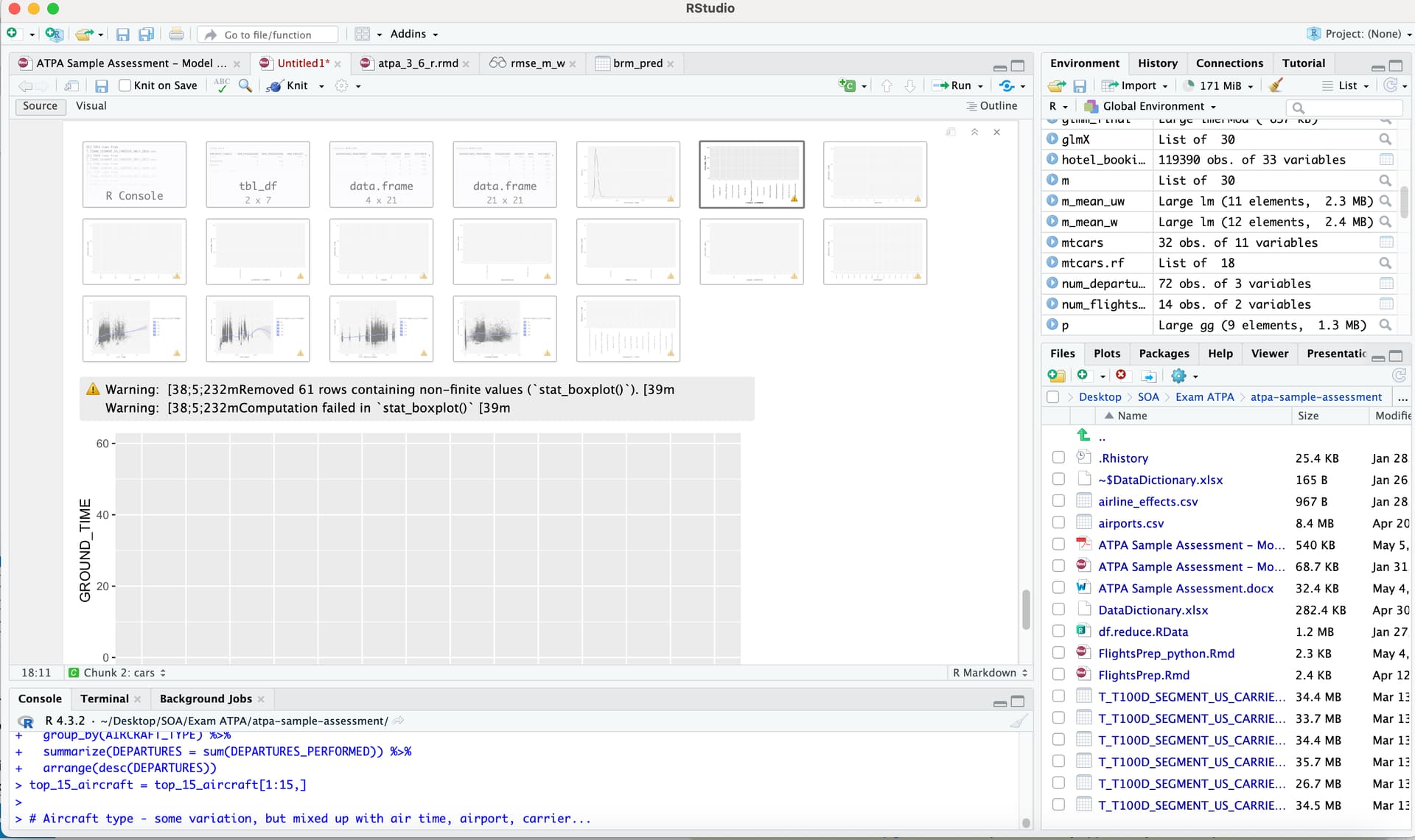
however, I have just run your code but some of the graphs cannot be shown still (as shown in my attachment)
I’m wondering if there’s anything wrong with my version of software since I guess most ppl are using windowOS
FYI, I m using version 2023.12.0+369(2023.12.0+369)on my MacBook
Not a problem. It was the only way I could even start to get a handle on the "real" code before the end of the year. It is the end of January:grinning:
Oh, wait a minute!
**Look at line 447. # library(quantreg) ** # Some users find they need this to see certain boxplots...if you get a blank boxplot, uncomment this and try again.
In any case I am hitting a problem at Chunk 37 where R freezes but I have not had a chance to fight my way through the verbiage.
Note I have fought my way through the jungle and I was not freezing. It is a Bayesian analysis ant STAN was successfully grinding away.
Here is a link to the code the complete stripped of all .rmd markers. It was too large to upload here.
I have accidentally left some redundant "summary" or print commands in. It was late.
Everything seems to be running okay on my machine: Ubuntu 22.04, R version 4.3.2 (2023-10-31), RStudio 2023.09.1+494 "Desert Sunflower" .
I have to admire whoever put this together at SOA. It is a brilliant simulation of how one would expect a newbie R programmer to work and exactly what someone could expect in an emergency. You may want to regard them as fiends and sadists but they do good work.
@jrkrideau recently I run many R codes (including some for package installation)
and when I run the above code, ive found the graphs can now be shown
I dunno know which exact code that solves the case
but may I ask one more question
what library code should I run for the geom_boxplot? is library(ggplot2) enough for running the box plot?