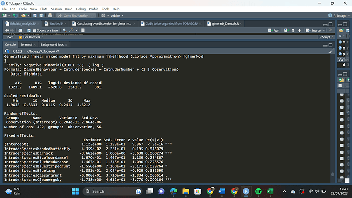
Hello! Please could someone help me with interpreting the output of a GLMM using a negative binomial family? I am writing a report and have no idea what my model is saying to me ![]()
Without a a reprex (see the FAQ, it's difficult to say anything useful about this specific model. There are two reasons:
-
Model evaluation can never be domain free, some idea of what the variables represent is necessary to keep analyst going off on a frolic and a folly based on what is recalled about a problem perhaps similar in its formal aspects but totally dis-similar in how it maps to the real world.
-
The economist's objection: Compared to what?
The following example is taken from the demo for lm.glm
dose <- c(1.6907, 1.7242, 1.7552, 1.7842, 1.8113, 1.8369, 1.861, 1.8839)
x <- c( 6, 13, 18, 28, 52, 53, 61, 60)
n <- c(59, 60, 62, 56, 63, 59, 62, 60)
(dead <- cbind(x, n-x))
#>       x
#> [1,]  6 53
#> [2,] 13 47
#> [3,] 18 44
#> [4,] 28 28
#> [5,] 52 11
#> [6,] 53  6
#> [7,] 61  1
#> [8,] 60  0
summary(     glm(dead ~ dose, family=binomial(link=logit)))
#>
#> Call:
#> glm(formula = dead ~ dose, family = binomial(link = logit))
#>
#> Coefficients:
#>             Estimate Std. Error z value Pr(>|z|)
#> (Intercept)  -60.717      5.181  -11.72   <2e-16 ***
#> dose          34.270      2.912   11.77   <2e-16 ***
#> ---
#> Signif. codes:  0 '***' 0.001 '**' 0.01 '*' 0.05 '.' 0.1 ' ' 1
#>
#> (Dispersion parameter for binomial family taken to be 1)
#>
#>     Null deviance: 284.202  on 7  degrees of freedom
#> Residual deviance:  11.232  on 6  degrees of freedom
#> AIC: 41.43
#>
#> Number of Fisher Scoring iterations: 4
summary(     glm(dead ~ dose, family=binomial(link=probit)))
#>
#> Call:
#> glm(formula = dead ~ dose, family = binomial(link = probit))
#>
#> Coefficients:
#>             Estimate Std. Error z value Pr(>|z|)
#> (Intercept)  -34.935      2.648  -13.19   <2e-16 ***
#> dose          19.728      1.487   13.27   <2e-16 ***
#> ---
#> Signif. codes:  0 '***' 0.001 '**' 0.01 '*' 0.05 '.' 0.1 ' ' 1
#>
#> (Dispersion parameter for binomial family taken to be 1)
#>
#>     Null deviance: 284.20  on 7  degrees of freedom
#> Residual deviance:  10.12  on 6  degrees of freedom
#> AIC: 40.318
#>
#> Number of Fisher Scoring iterations: 4
summary(z <- glm(dead ~ dose, family=binomial(link=cloglog)))
#>
#> Call:
#> glm(formula = dead ~ dose, family = binomial(link = cloglog))
#>
#> Coefficients:
#>             Estimate Std. Error z value Pr(>|z|)
#> (Intercept)  -39.572      3.240  -12.21   <2e-16 ***
#> dose          22.041      1.799   12.25   <2e-16 ***
#> ---
#> Signif. codes:  0 '***' 0.001 '**' 0.01 '*' 0.05 '.' 0.1 ' ' 1
#>
#> (Dispersion parameter for binomial family taken to be 1)
#>
#>     Null deviance: 284.2024  on 7  degrees of freedom
#> Residual deviance:   3.4464  on 6  degrees of freedom
#> AIC: 33.644
#>
#> Number of Fisher Scoring iterations: 4
anova(z, update(z, dead ~ dose -1))
#> Analysis of Deviance Table
#>
#> Model 1: dead ~ dose
#> Model 2: dead ~ dose - 1
#>   Resid. Df Resid. Dev Df Deviance
#> 1         6      3.446
#> 2         7    285.222 -1  -281.78
Created on 2023-07-24 with reprex v2.0.2
and it shows three model of some dose/mortality data, which differ in their diagnostic measures so that there is some basis to prefer one over the other. For example, they differ in their NULL deviance. This model has nothing to compare against.
This topic was automatically closed 42 days after the last reply. New replies are no longer allowed.
If you have a query related to it or one of the replies, start a new topic and refer back with a link.
