I finalized one version of a ggtree plot for a dataset of 300 samples, I made so based on the variety for this plant I colored the branches and tip labels (see figure below)
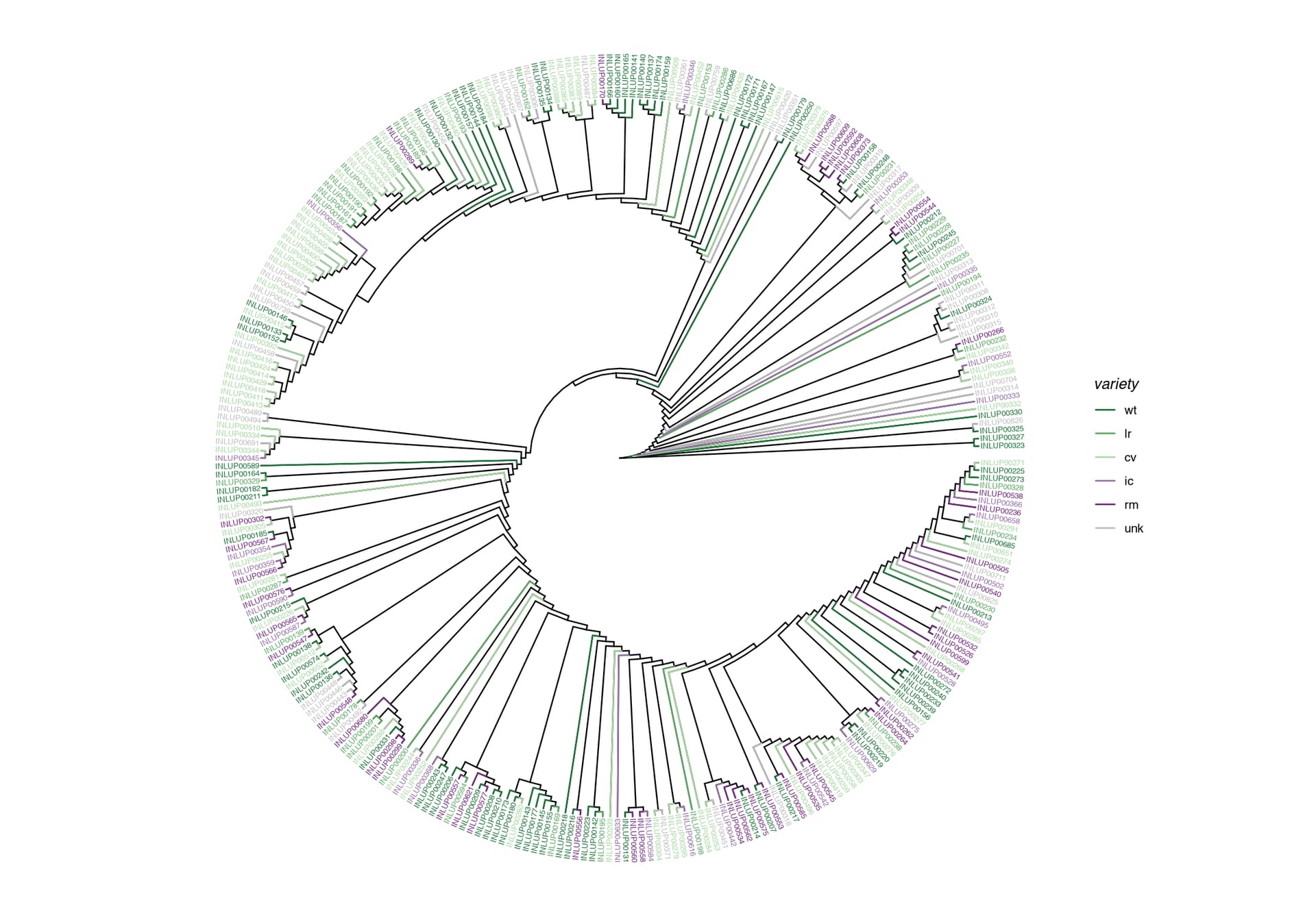
However, I wish to add another layer of information in the form of the location from where these samples have been collected — similarly to what has been done here for clades (e.g. an external strip for each location and an internal geom_cladelab for each variety the same color as the branches and tip labels).
I can't quite get the mechanics of how to do so... although it seems quite intuitive I must be getting something wrong. Thanks in advance for any help or suggestion!
MWE
library(ape)
library(scico)
library(tidyr)
library(dplyr)
library(tibble)
library(ggtree)
library(treeio)
library(ggplot2)
library(forcats)
library(phangorn)
library(tidytree)
library(phytools)
library(phylobase)
library(TreeTools)
library(ggtreeExtra)
library(RColorBrewer)
library(treedata.table)

###LOAD DATA AND WRANGLING
ibs_matrix = read.delim("/path/to/phylo_tree_header_ibs.phy", sep="\t", header=TRUE)
#colnames(ibs_matrix)[1] <- ""
#ibs_matrix[1] <- NULL

ibs_matrix_t <- t(ibs_matrix)


###ADD META INFO AND DF FORMATTING
variety <-  c("wt", "wt", "lr", "lr", "cv", "cv")

location <- c("ESP", "ESP", "ESP", "ITA", "ITA", "PRT")

meta_df <- data.frame(ibs_matrix_t[, 1], variety, location); meta_df <- meta_df[ -c(1) ]
meta_df$id <- rownames(meta_df); meta_df <- meta_df[,c(3,1,2)]
rownames(meta_df) <- NULL

lupin_UPGMA <- upgma(ibs_matrix_t) #roted tree

meta_df$variety <- factor(meta_df$variety, levels=c('wt', 'lr', 'cv'))

###BASIC PLOT
t2 <- ggtree(lupin_UPGMA, branch.length='none', layout="circular") %<+% meta_df + geom_tree(aes(color=variety)) + geom_tiplab(aes(color=variety), size=2) +
  scale_color_manual(values=c(brewer.pal(11, "PRGn")[c(10, 9, 8)], "grey"), na.translate = F) +
  guides(color=guide_legend(override.aes=aes(label=""))) +
  theme(legend.title=element_text(face='italic'))
t2

###ADD CLADES AND STRIPS
#not sure if needed
lupin_UPGMA2 <- as_tibble(lupin_UPGMA); colnames(lupin_UPGMA2)[4] <- "id"; lupin_UPGMA2 <- full_join(lupin_UPGMA2, meta_df, by="id")

#again not sure whether missing are supported...
lupin_UPGMA2 <- lupin_UPGMA2 %>%
  mutate_if(is.character, ~replace_na(.,"")) %>%
  mutate_if(is.numeric, replace_na, replace=0) %>%
  mutate(variety=fct_na_value_to_level(variety, ""))
lupin_strip <- as_tibble(lupin_UPGMA2) %>% dplyr::group_split(location)

#test on a small subset of groups
t2_loc <- t2 +

geom_cladelab(
    data = lupin_strip[[1]],
    mapping = aes(
    node=parent,
    label=location,
    color=location
    ),
    offset = 1.4,
    offset.text = .5,
    barcolor = "darkgrey",
    fontface = 3,
    align = TRUE
) +

geom_cladelab(
    data = lupin_strip[[2]],
    mapping = aes(
      node=parent,
      label=location,
      color=location
    ),
    offset = 1.4,
    offset.text = .5,
    barcolor = "darkgrey",
    fontface = 3,
    align = TRUE
) +

geom_strip(1, 6, color = "darkgrey", align = TRUE, barsize = 2,
             offset = 1.4, offset.text = 1.5, parse = TRUE)
t2_loc
DPUT ibs_matrix – 6 samples only
structure(list(INLUP00130 = c(0, 0.0989238, 0.0866984, 0.0890377,
0.0914165, 0.0931102), INLUP00131 = c(0.0989238, 0, 0.0960683,
0.0940636, 0.0947124, 0.0919737), INLUP00132 = c(0.0866984, 0.0960683,
0, 0.0859928, 0.0892208, 0.0946745), INLUP00133 = c(0.0890377,
0.0940636, 0.0859928, 0, 0.0838224, 0.0890456), INLUP00134 = c(0.0914165,
0.0947124, 0.0892208, 0.0838224, 0, 0.0801982), INLUP00135 = c(0.0931102,
0.0919737, 0.0946745, 0.0890456, 0.0801982, 0)), row.names = c(NA,
6L), class = "data.frame")