ggplot2 map of Canada with labels, shapefile issue

[lids]

Hello,

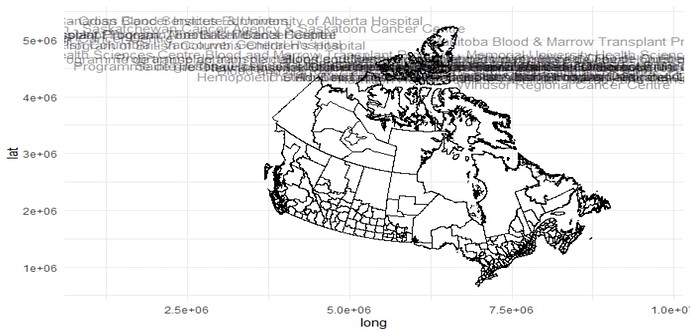
I am trying to create a map of Canada using ggplot2 that I can add labels to. I would like to label the location of specific treatment centers, mostly located in major cities.

I used the StatsCan census subdivisions cartographic boundary file (2016 Census Boundary files) to produce a map of Canada.

#shapefile
s_census <- shapefile("~/data/lcd_000b16a_e.shp")
s_census_fortified <- tidy(s_census)

map
ggplot(data = s_census_fortified,
aes(x = long, y = lat, group = group, fill = "id")) +
geom_polygon(color = "black", fill = "white", size = 0.1) +
guides(fill = "none") +
theme_minimal()

Next I try to use geom_text to label specific locations on the map pulled from a separate file called mapdata_AML. The long and lat in this file were manually extracted from Google using street address information.

ggplot(data = s_census_fortified, aes(x = long, y = lat, group = group, fill = "id")) +
geom_polygon(color = "black", fill = "white", size = 0.1) +
guides(fill = "none") +
geom_text(data = mapdata_AML, aes(label = Centre, x = long, y = lat, group = group),
label.padding = unit(0.55, "lines"),
label.size = 0.35,
color = "black",
fill="gray90", alpha = 0.4 ) +
theme_minimal()

But all of the labels are off the map. I don't understand why there is no overlap between my label file and the shapefile.

Can anyone help? Have I done something wrong with the shapefile import and transformation?

Thank you.

[williaml]

I haven't downloaded your file, but join the shapefile to the data file, then plot.

[jrmuirhead]

Hi @lids and welcome!

We don't have a copy your mapdata_AML file, so it's hard to troubleshoot.

What's happening is that your basemap s_census and your locations mapdata_AML are in two different Coordinate Reference Systems (CRS). The s_census data has coordinate system PCS_Lambert_Conformal_Conic (EPSG 3347) (units are in meters), and your mapdata_AML file has longitude and latitude probably in EPSG 4326 (units are in degrees).

You will either have to transform mapdata_AML to match the basemap, or vice versa.

Here's an example using simple features

library("sf")
library("here")
library("ggplot2")

s_census <- st_read(here("data", "lpr_000b16a_e.shp"))
# Projected CRS: PCS_Lambert_Conformal_Conic (EPSG 3347)

map_aml <- st_as_sf(map_aml, coords = c("long", "lat"),
  crs = st_crs(4326)) 

map_aml <- st_transform(map_aml,  crs = 3347)

census_map <- ggplot() +
  geom_sf(s_census) +
  geom_sf(map_aml) +
  coord_sf()

[lids]

This is very helpful. Thank you, @jrmuirhead