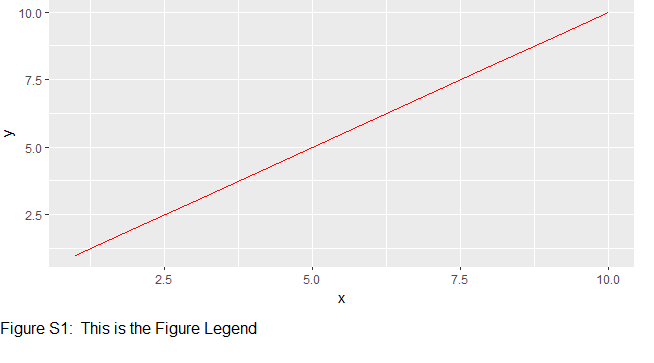
In creating a figure in a Supplement to a ms that I am submitting to a journal, I am instructed to "include the figure legend within the final graphic." I can think of two ways to do this.
a. I can add annotation text below the bottom of the graphic, possibly in a wide bottom plot margin.
b. If I can plot a text only plot, I can add it to the figure using grid.arrange(). But I can't find instructions on creating a text only plot.
Can someone point me to a URL that explains how to add a text figure legend below a plot using ggplot2?
Thanks in advance for the help.
Larry Hunsicker
You can annotate plots directly using the annotate() function (part of ggplot2), here is a link to the documentation of that function.
The tableGrob and grid.table functions in the gridExtra package might be helpful. Here's a Stack Overflow question that deals with adding a table grob beneath a ggplot. Also, the answers to this Stack Overflow question, although not addressed directly to your problem, might give you some ideas about how to proceed.
There are probably several ways to get what you're looking for, but we'll likely need more information to provide concrete guidance and code. Could you provide a reproducible example (with fake data, if necessary), or at least a drawing that will give us an idea of how the plot and legend are supposed to look?
cowplot also has tools that let you arrange and layer a wide variety of different things into a plot, and I find the learning curve gentler than gridExtra. See the intro vignette:
https://cran.r-project.org/web/packages/cowplot/vignettes/introduction.html
However, before you go down any of these paths — if I were given this constraint, I would probably just output a PDF via R Markdown (maybe with a non-letter page size) that had my plot and legend, and supply that as "the figure". Do you have a specific figure file type you are required to use? The PDF can be converted into any other image type as a separate step (e.g., via ImageMagick or magick).
An extremely basic example (I heroically resisted following the LaTeX  any further
  ) :
) :
---
output:
  pdf_document:
    fig_width: 8
    fig_height: 6
geometry:
  - paperwidth=8.125in
  - paperheight=6.125in
  - hmargin=0.125in
  - vmargin=0.125in
header-includes:
  - \pagenumbering{gobble}
---

```{r pressure, echo=FALSE}
plot(pressure)
```

**Figure 1.** Sapiente velit a voluptatibus provident in omnis. Soluta quas ipsa nemo ut
hic sit ratione tempora. Unde cupiditate nihil est repudiandae repellat quisquam illo
suscipit. Autem quisquam quibusdam numquam aut. Soluta expedita rem et qui ut quo
officia quam. Eius totam ad quisquam illo debitis fugit.
Example magick lines to take the output and convert into jpeg (assuming the Rmd was called plot_with_legend):
plot_legend <- magick::image_read("plot_with_legend.pdf", density = 300)
magick::image_write(plot_legend, "plot_with_legend.jpg", format = "jpeg", quality = 85, density = 300)
Jim89: Annotate() puts the legend into the plot. If you try to place the legend below the plot using a negative y position, ggplot extends the y-axis downward, but the legend is still within the plot.
I may have been unclear. I did not mean to insert the usual sort of plot legend into the plot. Rather, when one publishes a paper in a scientific journal, each plot needs what is called by the publishers a "Legend" that is placed immediately below the graphic and lets the reader know what the plot shows -- not we normally mean by a plot legend.
See my reply below to joels. Thanks for your suggestion
Joels: tableGrob has got me most of the way to what I need. Let me show you what I hope to get:
df1 <- data.frame(x = 1:10, y = 1:10)
p <- ggplot(df1, aes(x = x, y = y)) + geom_line(col = 'red')
FigLegend1 <- data.frame(legend = "Figure S1: This is the Figure Legend")
g <- tableGrob(FigLegend1, rows = NULL, cols = NULL)
b <- arrangeGrob(p, g, nrow = 2, heights = unit(c(2, .25),c("null", "null")))
plot(b)
This gives me:
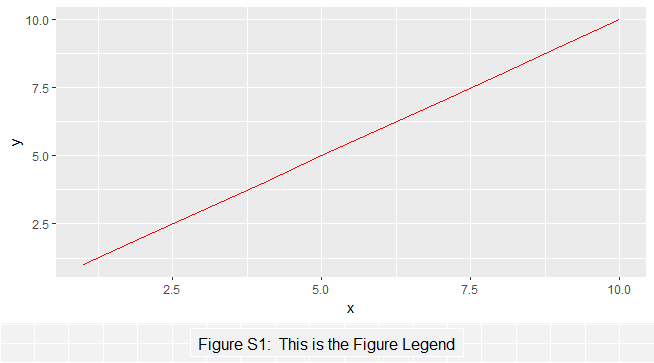
Now I need to get a blank background for the tableGrob and left justify the text. It would be nice, too, to be able to control the font size.
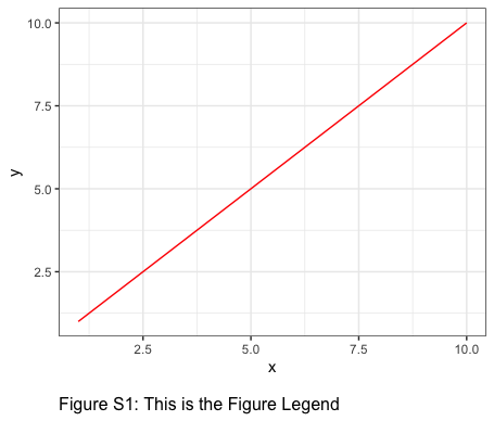
Based on your example, would a caption do what you need? For example:
p +
  labs(caption="Figure S1: This is the Figure Legend") +
  theme(plot.caption=element_text(size=12, hjust=0, margin=margin(15,0,0,0)))
To get rid of the gray background, use ttheme_minimal() when creating the table (which also allows you to set the font size) and use grid.draw instead of plot when rendering it. To left justify the table, I've added a null grob as a spacer on the right to push the table to the left (there's probably a better way):
g <- tableGrob(FigLegend1, rows = NULL, cols = NULL,
               theme=ttheme_minimal(core=list(fg_params=list(fontsize=12))))
b <- arrangeGrob(p,
                 arrangeGrob(g, nullGrob(), widths=c(1,1)),
                 nrow = 2, heights = unit(c(2, .25),c("null", "null")))
grid.newpage()
grid.draw(b)
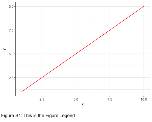
As I was working on this, I realized that you don't need tableGrob if all you want is some text. If you want to add a separate grob with just text (as opposed to using the caption feature of ggplot as described in my earlier answer), you can use textGrob from the grid package. With textGrob you can also get exact horizontal positioning of the text relative to the plot:
FigLeg = textGrob("Figure S1: This is the Figure Legend",
                  x = 0.01,
                  just="left",
                  gp=gpar(fontsize=12))

b <- arrangeGrob(p, FigLeg,
                 nrow = 2, heights = unit(c(2, .25),c("null", "null")))

grid.newpage()
grid.draw(b)
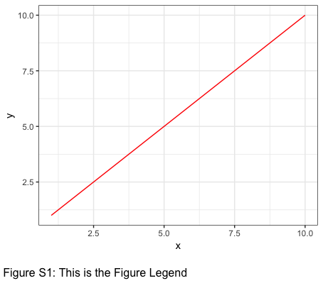
YES!! I actually thought of using textGrob. (I guessed that if there was a tableGrob, there must be a textGrob, too.) I made room at the bottom of the graphic using theme(plot.margin), and then added the textGrob. I suspect that this is basically what the theme(plot.caption) does. My result is lot like yours.
p <- ggplot(df1, aes(x = x, y = y)) + geom_line(col = 'red')+
theme(plot.margin = unit(c(0, 1, 3, 0), "lines"))
p
grid.text("Figure S1: This is the Figure Legend",
x = unit(0, "npc"), y = unit(.1, "npc"), just = "left")
Many thanks for the help!
Hi there! If your question's been answered, would you mind choosing a solution? It helps other people see which questions still need help, or find solutions if they have similar problems. Here’s how to do it:
