GGplot - Test Information Functions for multiple groups

Hello,
I am having trouble getting ggplot to recognise and plot multiple groups on TIFs. I have three groups (early, middle, and late) and would like to compare two at a time on three different plots. However, I am repeatedly getting an error with the groups.
I am guessing that the original function does not account for groups, and instead generates the function for the whole sample.
Here is how I am creating the grouping variable:

group <- c(rep('Early', sum(dat$age == "Age 18-30")), 
           rep('Middle', sum(dat$age == "Age 31-49")),
           rep('Late', sum(dat$age == "Age 50+")))

The code used is below..:

# test_info() is used to get the information
(mirt(newdat, 1, pars = 'values'))
mod <- mirt(newdat, 1)
Theta <- matrix(seq(-6,6,.01))
testinfo(mod, Theta, group, individual = FALSE,
         which.items = 1:extract.mirt(mod, "nitems"))
tI <- testinfo(mod, Theta, group=group)
se<- 1/(sqrt(tI)) #get the standard error
tI<- cbind.data.frame(tI,seq(-6,6,length.out=1201), se) #1201 points here, since looking at info by .01 from theta -6 to +6
colnames(tI) <- c("information", "xAxis","se")

### Plot the groups [change label as needed]:
p1 <- ggplot(tI, aes(x=xAxis, y=information, group=groups, colour="black")) + geom_line()  + theme_bw() +
  scale_colour_identity(name="", guide="legend", labels=c("Early")) +
  theme(panel.grid.major = element_blank(), panel.grid.minor = element_blank(),
        panel.background = element_blank(), axis.line = element_blank(),
        axis.text=element_text(size=14),
        axis.title=element_text(size=14),
        legend.text=element_text(size=14),
        legend.title=element_text(size=14),
        plot.title = element_text(hjust = 0.5, size=16, face="bold"),
        legend.position="bottom") +
  labs(x="\nθ", y = "Information\n") +
  scale_x_continuous(breaks=c(-6,-4,-2,0,2,4,6)) +ggtitle("Test Information Curve\n")

...with the command causing the error here:

# extract gtable:
g1 <- ggplot_gtable(ggplot_build(p1)) 
# Error: Aesthetics must be either length 1 or the same as the data (1201): group

Any help would be greatly appreciated :slightly_smiling_face:

Hi @baglolese. Can you provide some sample data that can be used to test the code or at least provide the sample data of tI data frame for testing the ggplot code.

Hi @raytong,

Certainly -- I've attached some sample data, n = 300 for each of three groups. The data is uploaded here: https://easyupload.io/f329qu

Thank you for your assistance with this!

@baglolese. I am not familiarise with the mirt package. But according to the documentation, you should use the multipleGroup function. By my guess, I suggest the following code but I don't know if the setting is correct for your model.

library(haven)
library(tidyverse)
library(mirt)

newdat <- read_sav("Downloads/IRTsampledata.sav")

group <- c(rep('Early', sum(newdat$age == "1")),
           rep('Middle', sum(newdat$age == "2")),
           rep('Late', sum(newdat$age == "3")))

group <- factor(group, levels = c("Early", 'Middle', "Late"))

Theta <- matrix(seq(-6,6,.01))
mg <- multipleGroup(newdat[,-1], mirt.model('F1 = 1-20'), group)

tI <- map_dfr(1:3, ~{
  groups <- c("Early", 'Middle', "Late")
  ti <- testinfo(mg, Theta, group = .x)
  data.frame(information = ti, xAxis = Theta, se = 1/(sqrt(ti)), group = groups[.x], stringsAsFactors = FALSE)
})

p1 <- ggplot(tI, aes(x=xAxis, y=information, group=group, colour="black")) + geom_line()  + theme_bw() +
  scale_colour_identity(name="", guide="legend", labels=c("Early")) +
  theme(panel.grid.major = element_blank(), panel.grid.minor = element_blank(),
        panel.background = element_blank(), axis.line = element_blank(),
        axis.text=element_text(size=14),
        axis.title=element_text(size=14),
        legend.text=element_text(size=14),
        legend.title=element_text(size=14),
        plot.title = element_text(hjust = 0.5, size=16, face="bold"),
        legend.position="bottom") +
  labs(x="\nθ", y = "Information\n") +
  scale_x_continuous(breaks=c(-6,-4,-2,0,2,4,6)) +ggtitle("Test Information Curve\n")

g1 <- ggplot_gtable(ggplot_build(p1))

Hi @raytong,

Thank you for your suggestions. The code you provided has generated the function, my thanks!
If I may ask, how can I specify a legend (identifiers for each Early, Middle, etc.) and line type ("solid", "dashed", "dotted")? At the moment, the legend only specifies one of the three solid lines as Early.

Thanks again

@baglolese. You may change the ggplot function as follow.

ggplot(tI, aes(x=xAxis, y=information, group=group, linetype=group))

@raytong

As I am making several plots, I would like to specify the linetypes for each group, so I can keep the line type consistent by group for each plot (i.e., Early always solid, Middle always dashed, and Late always dotted). This is because I am making three TIF plots from these three groups, with each group compared against another (Early and Middle, Early and Late, Middle and Late).

This is excellent as it stands -- I would just ideally like to make the line specifications above, and remove the extra 'Early' label as shown in the attached image, generated by my output:

@baglolese. You can add a named vector to scale_linetype_manual function to specify the line type. And factor the group column to arrange the order of group.

library(haven)
library(tidyverse)
library(mirt)

newdat <- read_sav("/Users/raytong/Downloads/IRTsampledata.sav")

group <- c(rep('Early', sum(newdat$age == "1")),
           rep('Middle', sum(newdat$age == "2")),
           rep('Late', sum(newdat$age == "3")))

group <- factor(group, levels = c("Early", 'Middle', "Late"))

Theta <- matrix(seq(-6,6,.01))
mg <- multipleGroup(newdat[,-1], mirt.model('F1 = 1-20'), group)

tI <- map_dfr(1:3, ~{
  groups <- c("Early", 'Middle', "Late")
  ti <- testinfo(mg, Theta, group = .x)
  data.frame(information = ti, xAxis = Theta, se = 1/(sqrt(ti)), group = groups[.x], stringsAsFactors = FALSE)
})

tI <- tI %>%
  mutate(group = factor(group, levels = c("Early", 'Middle', "Late")))

p1 <- ggplot(tI, aes(x=xAxis, y=information, group=group, linetype = group)) + geom_line()  + theme_bw() +
  scale_colour_identity(name="", guide="legend", labels=c("Early")) +
  theme(panel.grid.major = element_blank(), panel.grid.minor = element_blank(),
        panel.background = element_blank(), axis.line = element_blank(),
        axis.text=element_text(size=14),
        axis.title=element_text(size=14),
        legend.text=element_text(size=14),
        legend.title=element_text(size=14),
        plot.title = element_text(hjust = 0.5, size=16, face="bold"),
        legend.position="bottom") +
  labs(x="\nθ", y = "Information\n") +
  scale_x_continuous(breaks=c(-6,-4,-2,0,2,4,6)) +ggtitle("Test Information Curve\n") +
  scale_linetype_manual(values = c(Early = "solid", Middle = "dashed", Late = "dotted"))

g1 <- ggplot_gtable(ggplot_build(p1))

Dear @raytong,

This is it! Brilliant, thank you for all your help. However, it's odd in both the plot and my printed test information, the Middle and Late groups have switched places (in the plot I posted above, the Middle function showed the highest peak of test information, yet in this new one, the Late group is in its place):

What part of the code can I edit to only plot two of the three groups at once?

I also am not familiar with mirt, but could help with ggplot(), and was interested in trying to understand the issue. However, when I run the code @raytong posted with the data you posted, I get different plots from yours: In my case, 'Middle' is the lowest curve, followed by 'Early', and then 'Late':

Not sure what this means. Maybe the posted data changed? Or maybe there's a random element that made its way into collective code, but escaped notice? The curves are not only in a different order, but the intersection that appears in yours close to \theta = -1 between the lower two curves does not appear in mine.

@baglolese. The plot difference may due to the data that you used. And if you want to plot only two groups, you can filter the data frame tI first.

tI <- tI %>%
  mutate(group = factor(group, levels = c("Early", 'Middle', "Late"))) %>%
  filter(group %in% c("Early", "Late"))

I think I figured out the mystery of the label-changing behavior: The function multipleGroups() will determine a group ordering implicitly if the group vector is not a factor, and will use the factor level ordering otherwise. In your original post, @baglolese, you supplied the group labels as a character vector, so multipleGroups() implicitly ordered them alphabetically. Later, the factor structure is not
automatically incorporated into the table tI in @raytong's code, so must be restored before plotting.

Below is an annotated and modified version of @raytong's code that incorporates these observations; it's written from a didactic point of view since I wasn't sure how familiar you are with the tidyverse .

library(haven)
library(tidyverse)
library(mirt)

newdat <- read_sav("IRTsampledata.sav")
newdata %>% head()

# create 'group' factor for use with 'multipleGroup()'
## extract indices of age range labels
age_indices <- 
  newdat %>% 
  pull(age)
age_indices %>% head()
## use indices to create 'group' vector of new age range labels
groups <- c("Early", 'Middle', "Late")
group <- groups[age_indices]
## convert to factor: necessary for use with 'multipleGroup()' to avoid
##  order of groups being implicitly determined
group <- factor(group, levels = groups)

# alternative approach to creating 'group' factor in 'newdat' itself
newdat <-
  newdat %>%
  # extract original age range labels and indices
  mutate(age_range = as_factor(age, levels = 'labels')) %>%
  mutate(age_index = as_factor(age, levels = 'values'))
newdat %>% head()
## create column with new age range labels
newdat <-
  newdat %>%
  mutate(age_label =
           case_when(
             age_index == 1 ~ "Early",
             age_index == 2 ~ "Middle",
             age_index == 3 ~ "Late"
           )
         )
newdat %>% head()
## drop age_index and age_range columns, and reorder columns
newdat <-
  newdat %>%
  select(age_label, Item_1:Item_20)
newdat %>% head()
## extract age_label column data and compare with 'group'
group.dup <- newdat %>% pull(age_label)
all(group == group.dup)

# create multigroup object
mg <- 
  multipleGroup(
    newdat %>% select(-age_label),
    mirt.model('F1 = 1-20'), 
    group
  )
## check ordering used for 'group' values
mg@Data$groupNames

# create table of results
Theta <- matrix(seq(-6,6,.01))

tI <- map_dfr(1:3, ~{
  ti <- testinfo(mg, Theta, group = .x)
  tibble(
    information = ti, 
    xAxis = Theta, 
    se = 1/(sqrt(ti)), 
    group = groups[.x]
    )
})
tI %>% head()
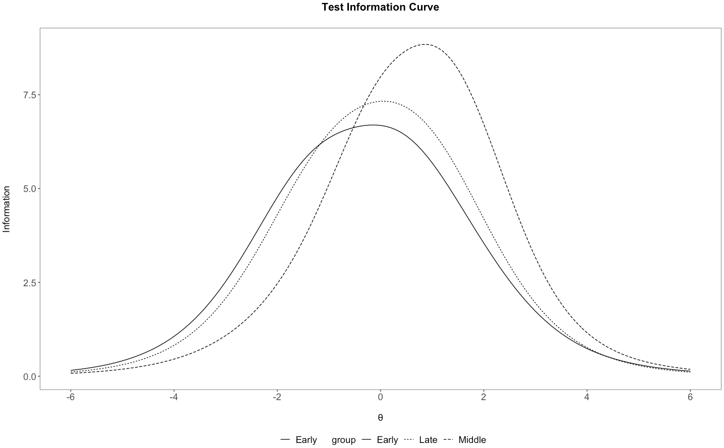
## Note: 'group' column is no longer a factor, so ggplot will use
##  alphabetical order implicitly in legend

# set theme for IRT plot separately
irt_theme <- 
  theme_bw() +
  theme(
    panel.grid.major = element_blank(), 
    panel.grid.minor = element_blank(),
    panel.background = element_blank(), 
    axis.line = element_blank(),
    axis.text=element_text(size=14),
    axis.title=element_text(size=14),
    legend.text=element_text(size=14),
    legend.title=element_text(size=14),
    plot.title = element_text(hjust = 0.5, size=16, face="bold"),
    legend.position="bottom"
  )

# create plot with 'tI' without converting 'group' to factor
tI %>% 
  ggplot(aes(x=xAxis, y=information)) +
  # add lines, one per group value, distinguished by line type
  geom_line(aes(linetype = group)) +
  irt_theme +
  # set labels and axis appearance
  labs(x="\nθ", y = "Information\n") +
  scale_x_continuous(breaks=c(-6,-4,-2,0,2,4,6)) +
  ggtitle("Test Information Curve\n")

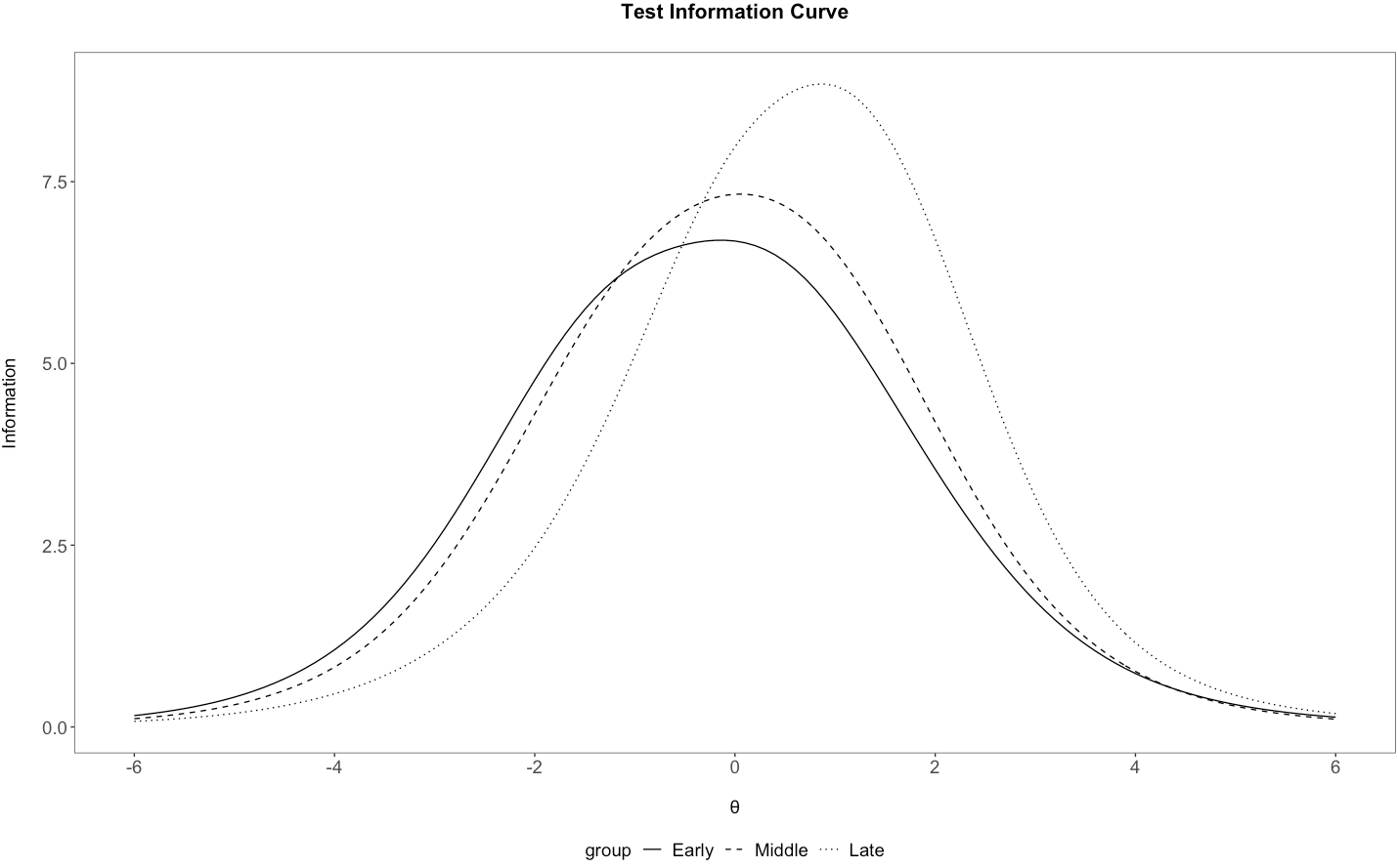
# create plot with 'tI', but converting 'group' to factor
## perform conversion in 'tI' itself
tI %>% 
  mutate(group = factor(group, levels = groups)) %>% 
  ggplot(aes(x=xAxis, y=information)) +
  geom_line(aes(linetype = group)) +
  irt_theme +
  labs(x="\nθ", y = "Information\n") +
  scale_x_continuous(breaks=c(-6,-4,-2,0,2,4,6)) +
  ggtitle("Test Information Curve\n")
## alternatively, perform conversion when building 'tI'
tI <- map_dfr(1:3, ~{
  ti <- testinfo(mg, Theta, group = .x)
  tibble(
    information = ti, 
    xAxis = Theta, 
    se = 1/(sqrt(ti)), 
    group = groups[.x] %>% factor(levels = groups)
  )
})
tI %>% head()

tI %>% 
  ggplot(aes(x=xAxis, y=information)) +
  geom_line(aes(linetype = group)) +
  irt_theme +
  labs(x="\nθ", y = "Information\n") +
  scale_x_continuous(breaks=c(-6,-4,-2,0,2,4,6)) +
  ggtitle("Test Information Curve\n")

# exclude 'Late' group
tI %>% 
  mutate(group = factor(group, levels = groups)) %>% 
  filter(group != 'Late') %>% 
  ggplot(aes(x=xAxis, y=information)) +
  geom_line(aes(linetype = group)) +
  irt_theme +
  labs(x="\nθ", y = "Information\n") +
  scale_x_continuous(breaks=c(-6,-4,-2,0,2,4,6)) +
  ggtitle("Test Information Curve\n")

Hi @dromano and raytong,

Thanks both for your great help with this. The filter command really helped in both your suggestions.

In # exclude Late group, I've added this line from raytong

scale_linetype_manual(values = c(Early = "solid", Middle = "dashed", Late = "dotted")

to keep linetype consistent, which was a main reason for switching to ggplot. I also increased line size in geomline()

geom_line(aes(linetype = group), size=1.2) 

to make them more visible scaled down.

Thanks again!

The sample code here is just a portion of the larger sample, so it makes sense your running it would provide different functions. Difference in organising of groups alphabetically or in order appears to have made the difference -- though I woudn't have expected the Late group to have the highest test information as they're the smallest group with by far the highest standard errors.

Now, on to making individual IIFs, ICCs, and TCCs!

I thought I'd add a last note! The scale_linetype_manual() allows you to specify exactly which labels get matched to which linetypes, but if all you want is a consistent matching, you could use this instead:

scale_linetype(limits = groups)

As a side effect, all three line types are preserved in the legend, which you could alter by adding the argument breaks = groups[-3] if you wanted to exclude 'Late'.

Good luck!

1 Like

I appreciate it! I hate to ask, but being new to tidyverse, I'm not sure how to begin editing this code to create test characteristic curves in a similar way.

No worries if you're unsure, you've done more than enough. Cheers!

I'm not familiar with test characteristic curves, but if you have non-tidyverse code that gets you part way there (like you started with here), I'm happy to see if I can help!

Great! I'm starting with a base code that looks something like this:

library(mirt)
library(ggplot2)
library(dplyr)
dat <- expand.table(LSAT7)
mod <- mirt(dat, 1, verbose=FALSE)

# Extract all items 
# Compute the probability trace lines
# Put into a list
traceline <- NULL
for(i in 1:length(dat)){
  extr.2 <- extract.item(mod, i)
  Theta <- matrix(seq(-4,4, by = .1))
  traceline[[i]] <- probtrace(extr.2, Theta)
}

# rename list
names(traceline) <- paste('item',1:length(traceline))

# rbind traceline
traceline.df <- do.call(rbind, traceline)

# create item names length based on length of theta provided
item <- rep(names(traceline),each=length(Theta))

# put them all together into a dataframe
l.format <- cbind.data.frame(Theta, item, traceline.df)


l.format$item<-as.factor(l.format$item)
aux<-l.format %>%
  group_by(item) %>%
  slice(which.min(abs(P.1-0.5))) # We are only using the P.1 column (dichotomous)

aux<-aux[order(aux$Theta),]
ord<-as.integer(aux$item)
l.format$item = factor(l.format$item,levels(l.format$item)[ord])

# plot chart
ggplot(l.format, aes(Theta, P.1, colour = item)) + 
  geom_line() + 
  ggtitle('Probability Tracelines') + 
  xlab(expression(theta)) + 
  ylab(expression(P(theta))) + 
  geom_hline(aes(yintercept = 0.5)) + theme_bw() + 
  theme(text = element_text(size=16),
        axis.text.x=element_text(colour="black"),
        axis.text.y=element_text(colour="black"),
        legend.title=element_blank())

I took a crack at it, but the traceline <- NULL command send back a group-related error.

The goal is to do ICCs and TCCs comparing the three groups, same as with the TIFs and some IIFs.

you probably want a traceline <- list() i.e. to have traceline be an empty list you can add things at the i index of , rather than a name not referencing an object (traceline <- NULL)

Hi @baglolese, would mind raising this in a separate question post? That way folks that search for similar answers will find a clear question-answer pair.