Ggplot label - advanced background

[Slavek]

Hi, I've been looking for solutions for a simple change I would like to do and I failed. Maybe you can help:

I would like to change labels background in my geom_line.

I can use my variable as factor like that:

geom_label(aes(label = scales::number(A2TB_mean, accuracy = 0.1), fill = factor(A2TB_mean)),
             color = 'white',
             show.legend = FALSE) +

but I don't know how to modify colour in this function (for example into red-amber-green scale where red is the lowest and green is the highest number). Currently, colours are random.

I even have issues with selecting my own colour as, despite selecting my own colour, my plot displays its default colour in the plot. In this example the colour is orange rather than "blue" I have specified:

 geom_label(aes(label = scales::number(A2TB_mean, accuracy = 0.1), fill="blue"),
             color = 'white',
             show.legend = FALSE) +

It must be something easy but all examples I have found are really basic and do not go into such detail of geom_label's sub-function.

Can you help giving solutions for option with the factor and option with my own colour?

Thank you in advance.

[technocrat]

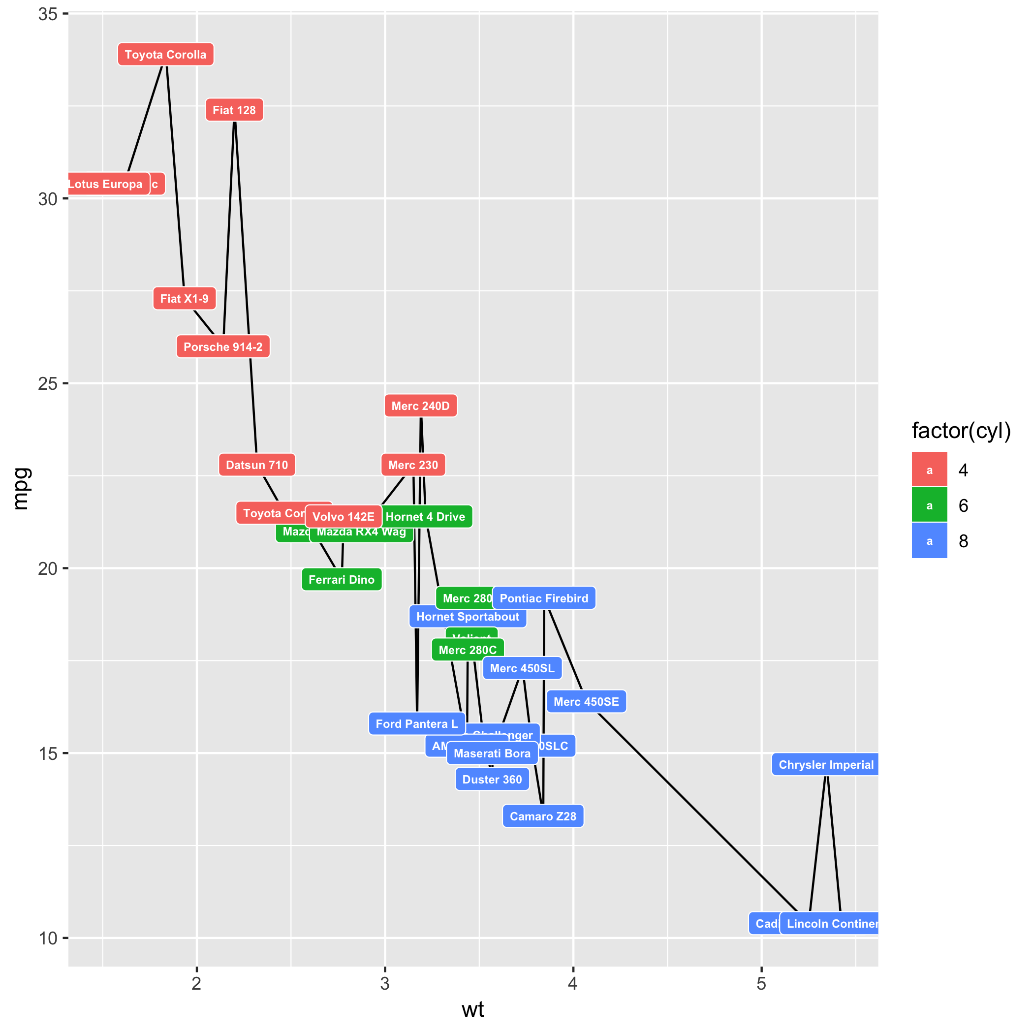
A reproducible example, called a reprex would get you a more focused answer, so I'll have to assume that you have something like

library(ggplot2)
library(RColorBrewer)
data(mtcars)

p <- ggplot(mtcars, aes(wt, mpg, label = rownames(mtcars))) + geom_line() + geom_label(aes(fill = factor(cyl)), colour = "white", fontface = "bold", size = 2)
p

^{Created on 2019-02-04 by the reprex package (v0.2.1)}

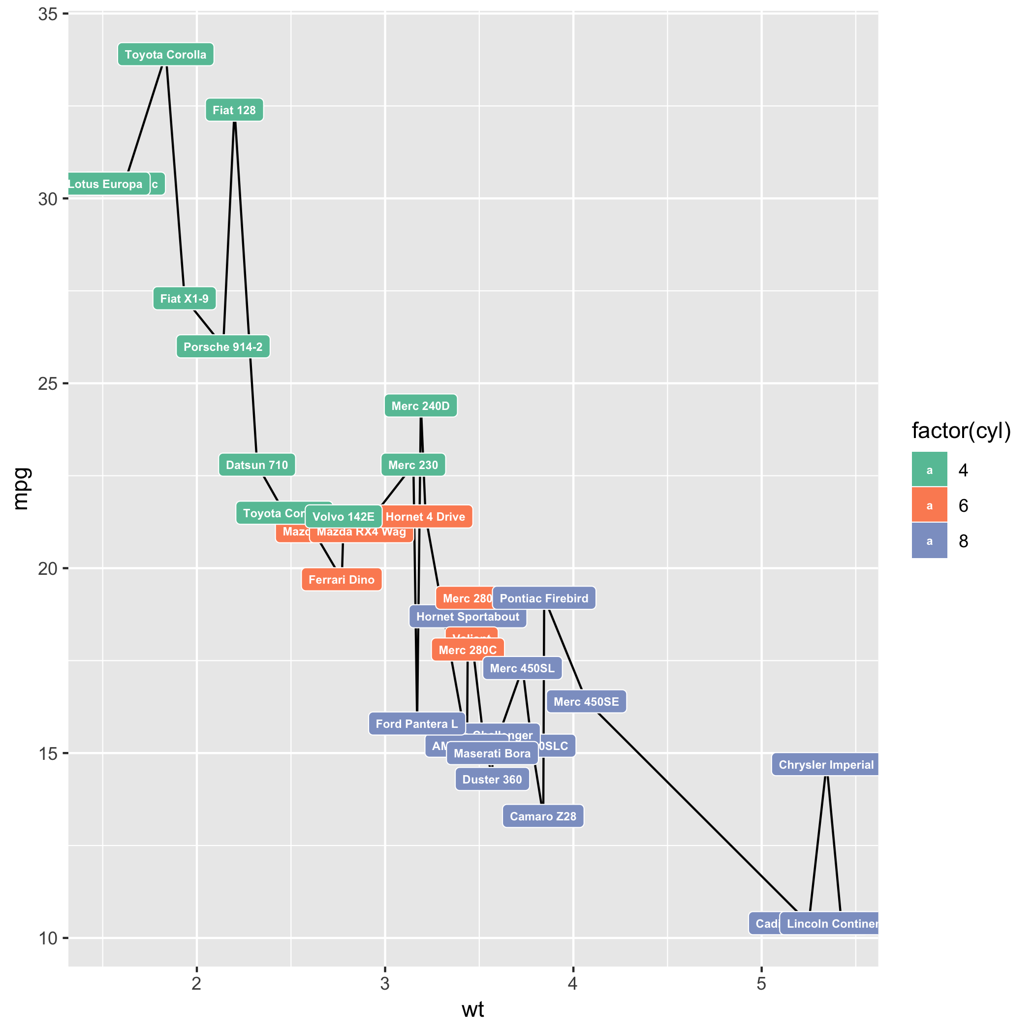
and you want to be able to do something like this

library(ggplot2)
library(RColorBrewer)
data(mtcars)

q <- ggplot(mtcars, aes(wt, mpg, label = rownames(mtcars))) + geom_line() + geom_label(aes(fill = factor(cyl)), colour = "white", fontface = "bold", size = 2) + scale_fill_brewer(palette = "Set2")
q

^{Created on 2019-02-04 by the reprex package (v0.2.1)}

Yes, you can, at the expense of hours of experiementation to find just the right colors. Also look at http://colorspace.r-forge.r-project.org

A more detailed explaination for color options (for maps, but the princples are similar) is my post at https://technocrat.rbind.io/2018/12/03/color-map-atlas-for-continuously-scaled-maps/

[andresrcs]

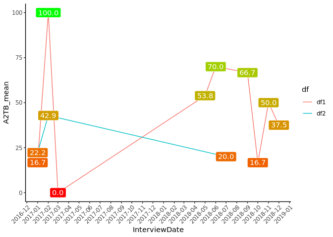
You can also use a continuos scale

geom_label(aes(label = scales::number(A2TB_mean, accuracy = 0.1), fill = A2TB_mean),
               color = 'white',
               show.legend = FALSE) +
    scale_fill_gradient(low = "red", high = "green") +

But I have to say that the result doesn't looks good to me

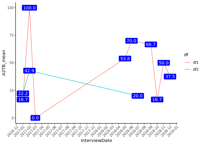
If you want a unique fill color, then take the fill argument out of the aes() statement

geom_label(aes(label = scales::number(A2TB_mean, accuracy = 0.1)),
               fill = "blue",
               color = 'white',
               show.legend = FALSE) +

[Slavek]

You are a genious!!!

Thank you

[Slavek]

I don't want to bother you too much but can you let me know where I could modify individual colours for each line and individual background for each label (for example blue for df1 and green for df2)?

[andresrcs]

You can do it with

scale_color_manual()
scale_fill_manual()

Read this secction of R4DS to learn how it works.

28 Graphics for communication | R for Data Science

[Slavek]

Thank you but there are two data frames therefore this issue is more problematic if I want fifferent colours for each...

[andresrcs]

Have you tried to understand the code that I gave you before? We have already merged the two dataframes into one, so there is no additional complication anymore.

library(dplyr)
library(tibbletime)
library(ggplot2)

df1_n <- df1 %>%
    select(InterviewDate, A2TB) %>% 
    mutate(InterviewDate = as.POSIXct(InterviewDate, tz = 'UTC'), df = 'df1')


df2_n <- df2 %>%
    select(InterviewDate, A2TB) %>% 
    mutate(InterviewDate = as.POSIXct(InterviewDate, tz = 'UTC'), df = 'df2')

df1_n %>% 
    rbind(df2_n) %>%
    arrange(InterviewDate) %>% 
    as_tbl_time(index = InterviewDate) %>%
    collapse_by("1 month", side = "start", clean = TRUE) %>%
    group_by(df, InterviewDate) %>%
    summarise(A2TB_mean = mean(A2TB, na.rm = TRUE))
#> # A time tibble: 12 x 3
#> # Index:  InterviewDate
#> # Groups: df [?]
#>    df    InterviewDate       A2TB_mean
#>    <chr> <dttm>                  <dbl>
#>  1 df1   2017-01-01 00:00:00      16.7
#>  2 df1   2017-02-01 00:00:00     100  
#>  3 df1   2017-03-01 00:00:00       0  
#>  4 df1   2018-05-01 00:00:00      53.8
#>  5 df1   2018-06-01 00:00:00      70  
#>  6 df1   2018-09-01 00:00:00      66.7
#>  7 df1   2018-10-01 00:00:00      16.7
#>  8 df1   2018-11-01 00:00:00      50  
#>  9 df1   2018-12-01 00:00:00      37.5
#> 10 df2   2017-01-01 00:00:00      22.2
#> 11 df2   2017-02-01 00:00:00      42.9
#> 12 df2   2018-07-01 00:00:00      20