Geom_text in facet_wrap

[Moritz]

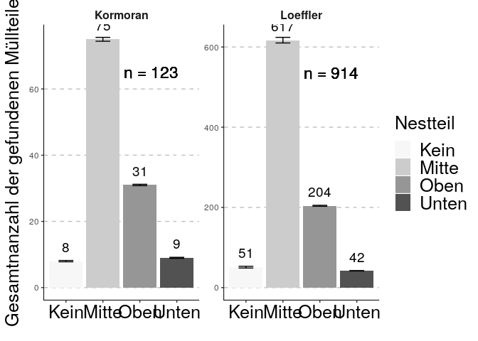
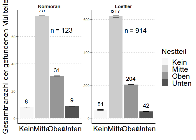
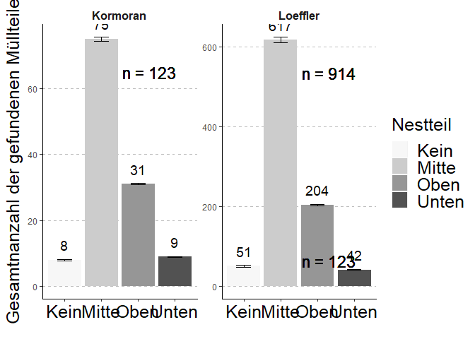
Hi I have a problem with my geom_text. My code and plot looks like this:

library(tidyverse)
library(reprex)
setwd("C:/Users/mroet/Desktop/reprex")
#Datensätze einlesen ----
Loeffler <-   read_delim("Loeffler_Gesamt1.CSV",";", escape_double = FALSE, trim_ws = TRUE)%>%   #Unbearbeitete Tabelle einladen
  gather(key = Kategorie, value = Anzahl, -Kolonie, -Nestnummer,-Nestteil, -Art, -Probe)   #Den Datensatz Tidy machen
#> Warning: Duplicated column names deduplicated: 'Fischkisten' =>
#> 'Fischkisten_1' [86], 'Hummerreusen' => 'Hummerreusen_1' [102]
#> Parsed with column specification:
#> cols(
#>   .default = col_double(),
#>   Art = col_character(),
#>   Kolonie = col_character(),
#>   Nestteil = col_character()
#> )
#> See spec(...) for full column specifications.

kormoran <-  read_delim("Kormoran_Gesamt1.CSV", ";", escape_double = FALSE, trim_ws = TRUE)%>%   #Unbearbeitete Tabelle einladen
  gather(key = Kategorie, value = Anzahl, -Nestnummer,-Nestteil, -Art)   #Den Datensatz Tidy machen
#> Warning: Duplicated column names deduplicated: 'Fischkisten' =>
#> 'Fischkisten_1' [84], 'Hummerreusen' => 'Hummerreusen_1' [100]
#> Parsed with column specification:
#> cols(
#>   .default = col_double(),
#>   Art = col_character(),
#>   Nestteil = col_character()
#> )
#> See spec(...) for full column specifications.
#Tabellen zusammenfügen ----
Gesamt <- bind_rows(Loeffler, kormoran, .id = NULL)

#Gesamtzahlen vergleichen ----

Vergleich <- Gesamt %>%
  group_by(Art, Nestteil, Nestnummer)%>%
  summarise(Anzahl = sum(Anzahl))%>%
  ungroup(Nestnummer)%>%
  group_by(Art, Nestteil)%>%
  mutate( Stab = sd(Anzahl), count = n(), se = (Stab/(sqrt(count))))%>%
  group_by(Stab, count, se, add=T)%>%
  summarise(Gesamt = sum(Anzahl))



plot_vergleich <- ggplot(Vergleich, aes(x = Nestteil, y = Gesamt, fill = Nestteil))+
  geom_bar(stat = 'identity', position = 'dodge')+
  geom_errorbar(aes( ymin = Gesamt - se, ymax = Gesamt + se ), width = .4)+
  geom_text(aes(label = Gesamt), size = 5,  position = position_dodge(0.8), vjust = -0.9)+
  geom_text(aes(x=3.3, y = 65), label = 'n = 123', size = 6)+
  geom_text(x=3.3, y =535, label = 'n = 914', size = 6)+
  scale_fill_brewer(name= 'Nestteil', palette = 'Greys')+
  labs(x ='', y = expression('Gesamtnanzahl der gefundenen Müllteile'))+
  facet_wrap(~Art, scales = 'free')+
  theme(panel.background = element_rect(fill = NA),
        panel.grid.major.y = element_line(color='grey', linetype = 20, size = 0.5),
        axis.line.x = element_line(linetype = 'solid'),
        axis.line.y = element_line(linetype = 'solid'),
        strip.background = element_blank(),
        strip.text = element_text(size = 12, face = 'bold'), 
        axis.text.x = element_text(size = 19, family = 'sans', colour = 'black'),
        axis.title.y = element_text(size = 19, family = 'sans', colour = 'black'),
        legend.text = element_text(size = 19,family = 'sans', colour = 'black'),
        legend.title = element_text(size = 19,family = 'sans', colour = 'black'))

plot_vergleich

^{Created on 2019-06-20 by the reprex package (v0.3.0)}

My problem is that I don't want the geom_text to appear on both sides. The "n=123" should only be at the left Grid and I don't know how to fix this. Is there an easy way to solve this problem? Thank you very much!

[andresrcs]

Could you turn this into a REPRoducible EXample (reprex) by providing some sample data? That would make things easier.

[Moritz]

Like this you mean?

library(tidyverse)
library(reprex)
setwd("C:/Users/Moritz Röttgen/Desktop/reprex")
#Datensätze einlesen ----
Loeffler <-   read_delim("Loeffler_Gesamt1.CSV",";", escape_double = FALSE, trim_ws = TRUE)%>%   #Unbearbeitete Tabelle einladen
  gather(key = Kategorie, value = Anzahl, -Kolonie, -Nestnummer,-Nestteil, -Art, -Probe)   #Den Datensatz Tidy machen
#> Warning: Duplicated column names deduplicated: 'Fischkisten' =>
#> 'Fischkisten_1' [86], 'Hummerreusen' => 'Hummerreusen_1' [102]
#> Parsed with column specification:
#> cols(
#>   .default = col_double(),
#>   Art = col_character(),
#>   Kolonie = col_character(),
#>   Nestteil = col_character()
#> )
#> See spec(...) for full column specifications.

kormoran <-  read_delim("Kormoran_Gesamt1.CSV", ";", escape_double = FALSE, trim_ws = TRUE)%>%   #Unbearbeitete Tabelle einladen
  gather(key = Kategorie, value = Anzahl, -Nestnummer,-Nestteil, -Art)   #Den Datensatz Tidy machen
#> Warning: Duplicated column names deduplicated: 'Fischkisten' =>
#> 'Fischkisten_1' [84], 'Hummerreusen' => 'Hummerreusen_1' [100]
#> Parsed with column specification:
#> cols(
#>   .default = col_double(),
#>   Art = col_character(),
#>   Nestteil = col_character()
#> )
#> See spec(...) for full column specifications.
#Tabellen zusammenfügen ----
Gesamt <- bind_rows(Loeffler, kormoran, .id = NULL)

#Gesamtzahlen vergleichen ----

Vergleich <- Gesamt %>%
  group_by(Art, Nestteil, Nestnummer)%>%
  summarise(Anzahl = sum(Anzahl))%>%
  ungroup(Nestnummer)%>%
  group_by(Art, Nestteil)%>%
  mutate( Stab = sd(Anzahl), count = n(), se = (Stab/(sqrt(count))))%>%
  group_by(Stab, count, se, add=T)%>%
  summarise(Gesamt = sum(Anzahl))

Vergleich
#> # A tibble: 8 x 6
#> # Groups:   Art, Nestteil, Stab, count [8]
#>   Art      Nestteil   Stab count    se Gesamt
#>   <chr>    <chr>     <dbl> <int> <dbl>  <dbl>
#> 1 Kormoran Kein      0.601     9 0.200      8
#> 2 Kormoran Mitte     3.19     30 0.583     75
#> 3 Kormoran Oben      1.16     30 0.212     31
#> 4 Kormoran Unten     0.837    30 0.153      9
#> 5 Loeffler Kein      6.63      9 2.21      51
#> 6 Loeffler Mitte    37.6      29 6.98     617
#> 7 Loeffler Oben      6.64     29 1.23     204
#> 8 Loeffler Unten     2.47     29 0.459     42

plot_vergleich <- ggplot(Vergleich, aes(x = Nestteil, y = Gesamt, fill = Nestteil))+
  geom_bar(stat = 'identity', position = 'dodge')+
  geom_errorbar(aes( ymin = Gesamt - se, ymax = Gesamt + se ), width = .4)+
  geom_text(aes(label = Gesamt), size = 5,  position = position_dodge(0.8), vjust = -0.9)+
  geom_text(aes(x=3.3, y = 65), label = 'n = 123', size = 6)+
  geom_text(x=3.3, y =535, label = 'n = 914', size = 6)+
  scale_fill_brewer(name= 'Nestteil', palette = 'Greys')+
  labs(x ='', y = expression('Gesamtnanzahl der gefundenen Müllteile'))+
  facet_wrap(~Art, scales = 'free')+
  theme(panel.background = element_rect(fill = NA),
        panel.grid.major.y = element_line(color='grey', linetype = 20, size = 0.5),
        axis.line.x = element_line(linetype = 'solid'),
        axis.line.y = element_line(linetype = 'solid'),
        strip.background = element_blank(),
        strip.text = element_text(size = 12, face = 'bold'), 
        axis.text.x = element_text(size = 19, family = 'sans', colour = 'black'),
        axis.title.y = element_text(size = 19, family = 'sans', colour = 'black'),
        legend.text = element_text(size = 19,family = 'sans', colour = 'black'),
        legend.title = element_text(size = 19,family = 'sans', colour = 'black'))

plot_vergleich

^{Created on 2019-06-20 by the reprex package (v0.3.0)}

The colum "Art" specifys the facet_wrap, the colum "Nestteil" is my x and the colum "Gesamt" is my y.
Now I want the sum of the colum "Gesamt" per species (colum "Art" these are two different species of birds) as a geom_text like "n = 123". The problem stays the same, the "n = 123" should just appear left. Hope you can understand my request better now. Thank you very much effort helping me out!

[Moritz]

Maybe you can use this code:

library(tidyverse)                          
test_plot <- tibble(Art = c('Kormoran','Kormoran','Kormoran','Kormoran','Loeffler','Loeffler','Loeffler','Loeffler'),
            Nestteil = c('Kein','Mitte','Oben','Unten','Kein','Mitte','Oben','Unten'),
            Gesamt = c(8,75,31,9,51,617,204,42),
            se = c(0.2003084,0.5827994,0.2116348,0.1527525,2.2110832,6.9807788,1.2322461,0.4591334))

^{Created on 2019-06-20 by the reprex package (v0.3.0)}

I hope it helps.

[andresrcs]

@Moritz

Like this you mean?

Not exactly, you are not providing sample data, we don't have access to your csv files, please read the link I gave you before.

[Moritz]

Sorry that was my fault. I think with this it should make it.

library(tidyverse)                          
test_plot <- tibble(Art = c('Kormoran','Kormoran','Kormoran','Kormoran','Loeffler','Loeffler','Loeffler','Loeffler'),
            Nestteil = c('Kein','Mitte','Oben','Unten','Kein','Mitte','Oben','Unten'),
            Gesamt = c(8,75,31,9,51,617,204,42),
            se = c(0.2003084,0.5827994,0.2116348,0.1527525,2.2110832,6.9807788,1.2322461,0.4591334))                     

plot_vergleich_test <- ggplot(test_plot, aes(x = Nestteil, y = Gesamt, fill = Nestteil))+
  geom_bar(stat = 'identity', position = 'dodge')+
  geom_errorbar(aes( ymin = Gesamt - se, ymax = Gesamt + se ), width = .4)+
  geom_text(aes(label = Gesamt), size = 5,  position = position_dodge(0.8), vjust = -0.9)+
  geom_text(aes(x=3.3, y = 65), label = 'n = 123', size = 6)+
  geom_text(x=3.3, y =535, label = 'n = 914', size = 6)+
  scale_fill_brewer(name= 'Nestteil', palette = 'Greys')+
  labs(x ='', y = expression('Gesamtnanzahl der gefundenen Müllteile'))+
  facet_wrap(~Art, scales = 'free')+
  theme(panel.background = element_rect(fill = NA),
        panel.grid.major.y = element_line(color='grey', linetype = 20, size = 0.5),
        axis.line.x = element_line(linetype = 'solid'),
        axis.line.y = element_line(linetype = 'solid'),
        strip.background = element_blank(),
        strip.text = element_text(size = 12, face = 'bold'), 
        axis.text.x = element_text(size = 19, family = 'sans', colour = 'black'),
        axis.title.y = element_text(size = 19, family = 'sans', colour = 'black'),
        legend.text = element_text(size = 19,family = 'sans', colour = 'black'),
        legend.title = element_text(size = 19,family = 'sans', colour = 'black'))

plot_vergleich_test

^{Created on 2019-06-20 by the reprex package (v0.3.0)}

[andresrcs]

This is not an elegant solution but It works

library(tidyverse)                          
test_plot <- tibble(Art = c('Kormoran','Kormoran','Kormoran','Kormoran','Loeffler','Loeffler','Loeffler','Loeffler'),
                    Nestteil = c('Kein','Mitte','Oben','Unten','Kein','Mitte','Oben','Unten'),
                    Gesamt = c(8,75,31,9,51,617,204,42),
                    se = c(0.2003084,0.5827994,0.2116348,0.1527525,2.2110832,6.9807788,1.2322461,0.4591334))                     

test_plot %>% 
    ggplot(aes(x = Nestteil, y = Gesamt, fill = Nestteil))+
    geom_bar(stat = 'identity', position = 'dodge')+
    geom_errorbar(aes( ymin = Gesamt - se, ymax = Gesamt + se ), width = .4)+
    geom_text(aes(label = Gesamt), size = 5,  position = position_dodge(0.8), vjust = -0.9)+
    geom_text(data = test_plot %>% filter(Art == "Kormoran"), x=3.3, y = 65, label = 'n = 123', size = 6) +
    geom_text(data = test_plot %>% filter(Art == "Loeffler"), x=3.3, y =535, label = 'n = 914', size = 6) +
    scale_fill_brewer(name= 'Nestteil', palette = 'Greys')+
    labs(x ='', y = expression('Gesamtnanzahl der gefundenen Müllteile'))+
    facet_wrap(~Art, scales = 'free')+
    theme(panel.background = element_rect(fill = NA),
          panel.grid.major.y = element_line(color='grey', linetype = 20, size = 0.5),
          axis.line.x = element_line(linetype = 'solid'),
          axis.line.y = element_line(linetype = 'solid'),
          strip.background = element_blank(),
          strip.text = element_text(size = 12, face = 'bold'), 
          axis.text.x = element_text(size = 19, family = 'sans', colour = 'black'),
          axis.title.y = element_text(size = 19, family = 'sans', colour = 'black'),
          legend.text = element_text(size = 19,family = 'sans', colour = 'black'),
          legend.title = element_text(size = 19,family = 'sans', colour = 'black'))

[aosmith]

This is a situation where I'd likely make a dataset for plotting the labels that has the faceting variable Art in it along with the axis position info and the labels. Here I create it manually, but sometimes we can do some of the work, like calculate sample size for the labels, via data summaries.

labeldat = data.frame(Art = c("Kormoran", "Loeffler"),
                      x = c(3.3, 3.3),
                      y = c(65, 535),
                      label = c("n = 123", "n = 914") )

Then text for each facet can be added in one geom_text() layer. Note this also gets rid of the issue of overplotting the text that happens when you don't use a new dataset for geom_text() and so the text is printed as many times as there are rows in the original data.

test_plot %>% 
    ggplot(aes(x = Nestteil, y = Gesamt, fill = Nestteil))+
    geom_bar(stat = 'identity', position = 'dodge')+
    geom_errorbar(aes( ymin = Gesamt - se, ymax = Gesamt + se ), width = .4)+
    geom_text(aes(label = Gesamt), size = 5,  position = position_dodge(0.8), vjust = -0.9)+
    geom_text(data = labeldat, mapping = aes(x = x, y = y, label = label, fill = NULL), size = 6) +
    scale_fill_brewer(name= 'Nestteil', palette = 'Greys')+
    labs(x ='', y = expression('Gesamtnanzahl der gefundenen Müllteile'))+
    facet_wrap(~Art, scales = 'free')+
    theme(panel.background = element_rect(fill = NA),
          panel.grid.major.y = element_line(color='grey', linetype = 20, size = 0.5),
          axis.line.x = element_line(linetype = 'solid'),
          axis.line.y = element_line(linetype = 'solid'),
          strip.background = element_blank(),
          strip.text = element_text(size = 12, face = 'bold'), 
          axis.text.x = element_text(size = 19, family = 'sans', colour = 'black'),
          axis.title.y = element_text(size = 19, family = 'sans', colour = 'black'),
          legend.text = element_text(size = 19,family = 'sans', colour = 'black'),
          legend.title = element_text(size = 19,family = 'sans', colour = 'black'))

Created on 2019-06-20 by the reprex package (v0.2.0).

[Moritz]

Thanks for your help!

[andresrcs]

If your question's been answered (even by you!), would you mind choosing a solution? It helps other people see which questions still need help, or find solutions if they have similar problems. Here’s how to do it:

FAQ: How do I mark a solution?

If your question has been answered, don't forget to mark the solution! How do I mark a solution? Find the reply you want to mark as the solution and look for the row of small gray icons at the bottom of that reply. Click the one that looks like a box with a checkmark in it: [image] Hovering over the mark solution button shows the label, "Select if this reply solves the problem". If you don't see the mark solution button, try clicking the three dots button ( ••• ) to expand the full set of options. When a solution is chosen, the icon turns green and the hover label changes to: "Unselect if this reply no longer solves the problem". Success! [solution_reply_author] …