geom_smooth with different spans per group

[ldecicco]

I have the same question that was asked here 3 years ago:

Using multiple values for span in geom_smooth in ggplot

The accepted answer doesn't seem to work (that is, changing the values in the span list don't make any difference to the plot)

# doesn't seem to work:
mtcars %>%
  ggplot(aes(x = wt,  y = mpg, color = factor(am))) +
  geom_point() +
  stat_smooth(geom = "smooth", 
              method = "loess", formula = y ~ x,
              method.args = list(span = c(0.2, 0.8)))

# works but is clunky:
ggplot() +
  geom_point(data = mtcars,
             aes(x = wt,  y = mpg, color = factor(am))) +
  geom_smooth(data = mtcars |> 
                filter(am ==1),
              aes(x = wt,  y = mpg, color = factor(am)),
              method = "loess", span = 0.2, 
              show.legend = FALSE) +
  geom_smooth(data = mtcars |> 
                filter(am == 0),
              aes(x = wt,  y = mpg, color = factor(am)),
              method = "loess", span = 0.8)

I have 2 related questions.

1. Is there a more streamlined way to use different spans for different groups of data other than looping through all the grouping levels?
2. Is there a good way to get the legend to show smoothing lines on only the data that has the smoothing line? Here's what I mean by that. Let's say we want to do this:

ggplot(data = mtcars,
       aes(x = wt,  y = mpg, color = factor(am))) +
  geom_point() +
  geom_smooth(data = mtcars |> 
                filter(am ==1),
              aes(x = wt,  y = mpg, 
                  color = factor(am), group = factor(am)),
              method = "loess", span = 0.5)

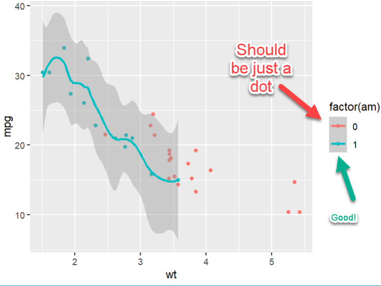
I think I could hack a custom legend together, but if there's some way to get it to work in a more legitimate way, that would be great to learn.

[technocrat]

Let's start with this

library(ggplot2)

# error bands obscure what is happening
ggplot(mtcars,aes(wt,mpg, color = factor(am))) +
  geom_point() +
  geom_vline(xintercept = 2.4) +
  geom_vline(xintercept = 3.6) +
  annotate("text",3,12,label = "OVERLAP") +
  geom_smooth(method =  "loess") +
  theme_minimal()
#> `geom_smooth()` using formula = 'y ~ x'

# removing them removes the overlaps of the
# error bands
ggplot(mtcars,aes(wt,mpg, color = factor(am))) +
  geom_point() +
  geom_smooth(method = "loess", se = FALSE) +
  theme_minimal()
#> `geom_smooth()` using formula = 'y ~ x'

^{Created on 2023-05-18 with reprex v2.0.2}

[ldecicco]

@ldecicco

span

Thanks for the example @technocrat I think I wasn't clear in my question. I'm trying to use different span values for the span argument in the geom_smooth function (I'd like to do something like span = c(0.2, 0.8)). This argument tells the lowess function how much to smooth. So for instance, if one of the "factor(am)" sets of data had a lot less points than the other, it might make sense to smooth them with different "span" values.

[technocrat]

Let's think about what the loess represents in these geoms.

The details are be found in the documentation for stats::loess(). The big picture is that we have two variables and are looking to visualize a function that gives a fit and we choose loess() because a linear fit isn't satisfactory, we want to show a non-linear fit, a curve that is able to continuously vary to reflect a varying relationship between the two variables.

All this time we are projecting on the Cartesian plane in 2-space.

The span argument provides a tuning parameter to vary the degree of smoothing in how the curve is fit by selecting the points to be used as the x axis varies.

Fitting is done locally. That is, for the fit at point xx , the fit is made using points in a neighbourhood of x , weighted by their distance from x (with differences in ‘parametric’ variables being ignored when computing the distance). The size of the neighbourhood is controlled by α (set by span or enp.target ). For α < 1α<1 , the neighbourhood includes proportion α of the points, and these have tricubic weighting (proportional to (1 - dist/maxdist)^3)^3. For α > 1α>1 , all points are used, with the ‘maximum distance’ assumed to be α^{1/p}α1/p times the actual maximum distance for p explanatory variables.

The default \alpha set with the span argument is 0.75, varying it toward one increases smoothness and toward zero decreases it. It does this in reference by weighting the distance of points from the fitted line. As far as i can tell, the weighting is linear, not quadratic or some other higher order. In any event, however, \alpha does not affect the weighting coefficient, but rather the span (distance of the x axis defining a neighboorhood. If it were possible to set multiple spans to account for points with differing attributes, there would need be some complication to account for overlapping spans. That can be provided by setting \alpha small enough so that no span contains points of more than one type. As a result, the curve would have the least possible smoothness.

In theory, we could fit a line in 3-space, where one variable is divided based on some attribute, but that's not loess does.

There is a weights parameter in loess(), but I honestly can't trace how it's used. loess is based on the S package cloess and I've looked at the source code for a later version, called dloess which is well commented but in terms of its Fortran statements, so it's difficult for me to follow because I failed to keep up after FORTRAN IV in the pre-System 360 days.

[ucfagls]

The GAM option for geom_smooth() would have this feature built in, except it would also choose the wiggliness (smoothing parameter, equivalent of the span hyperparameter in Loess). If that's not a problem, then:

library("ggplot2")

mtcars |>
  ggplot(aes(x = wt,  y = mpg, color = factor(am))) +
  geom_point() +
  geom_smooth(method = "gam", 
              formula = y ~ s(x),
              method.args = list(method = "REML"))

In this general there are nlevels(factor(ami)) GAMs here and in this particular data example two separate GAMs are fitted so if the data support it, you could have different wigglinesses for the two smooth functions fitted. Here though the data do not support non-linear functions so you have two estimated linear functions.

More generally, I would smooth data using the respective GAM and then plot:

library("mgcv")
library("gratia") # <- needs the dev version from github https://github.com/gavinsimpson/gratia#installing-gratia
library("dplyr")

mtcars2 <- mtcars |>
  mutate(am_f = factor(am))

m <- gam(mpg ~ am_f + s(wt, by = am_f),
  data = mtcars2, method = "REML")

# generate data for the two smooths
# this is a little clunky just now with the development version of gratia, but it works
ds0 <- mtcars2 |>
  filter(am_f == "0") |>
  data_slice(wt = evenly(wt))
ds1 <- mtcars2 |>
  filter(am_f == "1") |>
  data_slice(wt = evenly(wt))
ds <- bind_rows(ds0, ds1)

fv <- fitted_values(m, data = ds)

fv |>
  ggplot(aes(y = fitted, x = wt)) +
  geom_point(data = mtcars2, aes(y = mpg, x = wt, colour = am_f)) +
  geom_ribbon(aes(ymin = lower, ymax = upper, fill = am_f), alpha = 0.2) +
  geom_line(aes(colour = am_f))