I would strongly advise not to use the gam package over the mgcv package; the latter provides automatic smoothness selection whereas in the former you need to specify the degrees of freedom for the smooths. The blog post used the mgcv package, but you are misunderstanding the output there.
Note the formula that was used in that blog post:
medv ~ s(rm) + s(lstat) + ptratio + indus + crim + zn + age
Only two of the terms in this model are smooths: s(rm) and s(lstat). The other terms in the formula are parametric effects. That is why you see more entries in the Parametric coefficients table in the summary() output. There is nothing about rm and lstat in the Parametric coefficients table.
In your model, which should be specified as
DailyIncrease ~ s(Precipitation)
There is only a single model term and it is a smooth. As you have no parametric terms beyond the model constant term (the intercept), there will only be a single line in the Parametric coefficients table. The focus of inference should be on the smooth function itself and that is what is show in the Approximate significance of smooth terms table. Note that you shouldn't use df$var notation in model formulas; pass the df to the data argument in your model, hence
gam(DailyIncrease ~ s(Precipitation), data = preOutlierRem.dat, method = "REML")
or
gam(DailyIncrease ~ s(Precipitation), data = preOutlierRem.dat, method = "ML")
would be advised.
The smooth in your model is represented as a penalised thin plate spline; a spline is a function that is formed by a weighted sum of basis functions. Your spline was built using 9 thin plate spline basis functions. Each of those functions has a coefficient associated with it: run coef() on your model and you'll see the nine coefficients associated with the smooth, plus the intercept.
As the whole point of fitting a GAM is to estimate smooth functions, we should consider the estimates of those functions. There is little to no point in looking at the individual coefficients. This is why there is a single line in the model summary for the smooth; this is a Wald-like test against a null hypothesis that the true function is a flat, constant function with value 0 everywhere: \text{H}_0: f(x_i) = 0 \; \forall \; i.
Apart from that, we should plot the estimated smooth; you can do this with plot(model) using mgcv or use another package for plotting smooths fitted by mgcv, such as my gratia package or the itsadug package. With gratia you would just do draw(model) to get a nice ggplot-based version of the figure plot() would produce.
How do I find the estimate for the coefficient "Precipitation" in my model?
In summary, you don't; these models are not parameterised in the way you are expecting. There isn't a single coefficient for the smooth term. There are many coefficients associated with a smooth and it doesn't make sense in most cases to compare coefficients.
I want to be able to run two different GAM models and see how the estimate of the coefficient "Precipitation" varies between my two models.
This implies that you have the response variable DailyIncrease measured at two different conditions or settings. If so, you should fit one model, where we allow the smooth effect of the covariate on the response to differ between the two settings. The standard way to do this is shown below, in which I am assuming that you have joined your two data frames row-wise (into combined_dat) and that there is a variable prepostthat is a factor coding for whether we are using the pre or the post data set.
gam(DailyIncrease ~ prepost  + s(Precipitation, by = prepost),
  data = combined_dat, method = "REML")
This model fits two separate smooths, one where prepost == "pre" and one where prepost == "post"; you can then plot the two functions; with gratia::draw() or mgcv::plot.gam() for a visual comparison.
With this model there isn't a test for the difference. You can use gratia::difference_smooths() to compute a difference between the two estimated smooths and an associated uncertainty band. This can then be plotted to show where over the covariate the two functions differ.
An alternative model formulation is via an ordered factor, or via the sz basis. I'll show examples of these below.
Using your data I worked up the following example
Your original model
First load the data and packages we'll use. If you don't have gratia installed, follow the instructions here to install the development version
# packages
library("readr")
library("gratia")
library("mgcv")
library("dplyr")

# load data
pre  <- read_csv("PrecipDischargeOutliersRemPre.csv", col_types = "Ddddd-")
post <- read_csv("PrecipDischargeOutliersRemPost.csv", col_types = "Ddddd-")
Fit your original model, properly specified:
# original model
m_orig <- gam(DailyIncrease ~ s(Precipitation),
    data = pre, method = "REML")
The model summary is
# summary
summary(m_orig)
>  summary(m_orig)

Family: gaussian
Link function: identity

Formula:
DailyIncrease ~ s(Precipitation)

Parametric coefficients:
            Estimate Std. Error t value Pr(>|t|)
(Intercept) 0.068637   0.005005   13.71   <2e-16 ***
---
Signif. codes:  0 ‘***’ 0.001 ‘**’ 0.01 ‘*’ 0.05 ‘.’ 0.1 ‘ ’ 1

Approximate significance of smooth terms:
                   edf Ref.df     F p-value
s(Precipitation) 8.855  8.993 598.1  <2e-16 ***
---
Signif. codes:  0 ‘***’ 0.001 ‘**’ 0.01 ‘*’ 0.05 ‘.’ 0.1 ‘ ’ 1

R-sq.(adj) =  0.908   Deviance explained = 90.9%
-REML = -366.58  Scale est. = 0.013678  n = 546
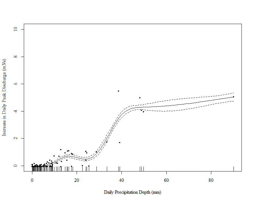
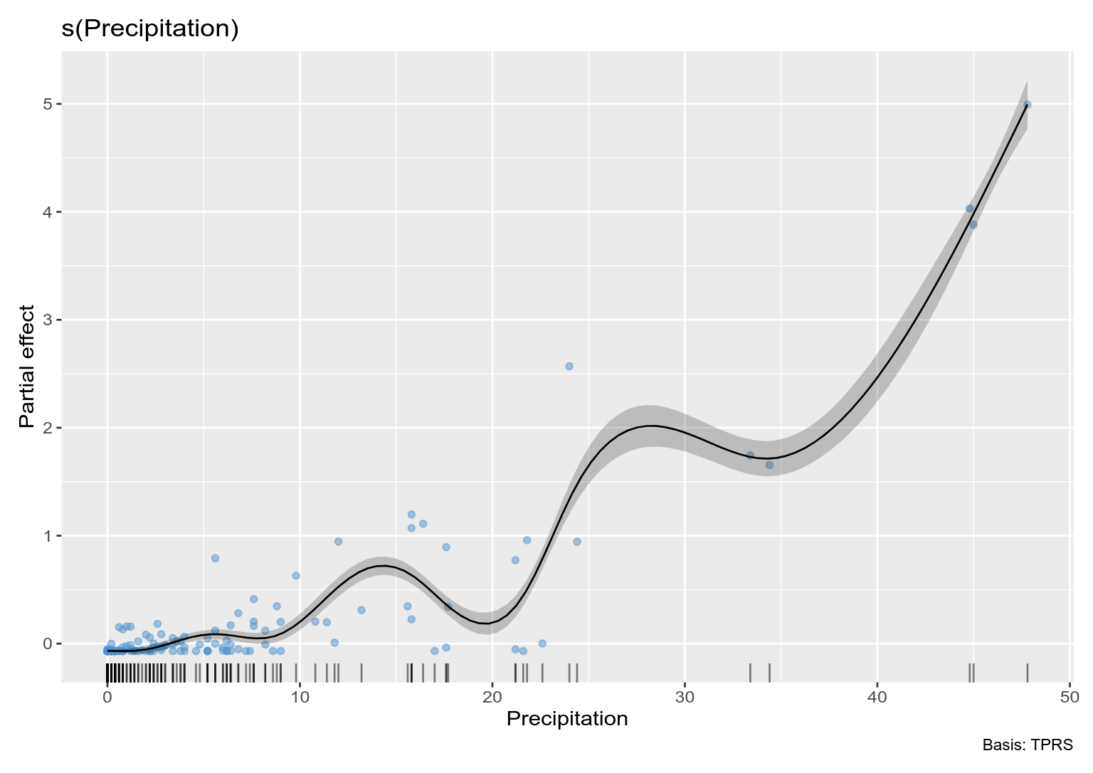
and plot the estimated smooth
# plot
draw(m_orig, residuals = TRUE)
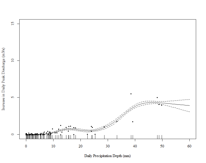
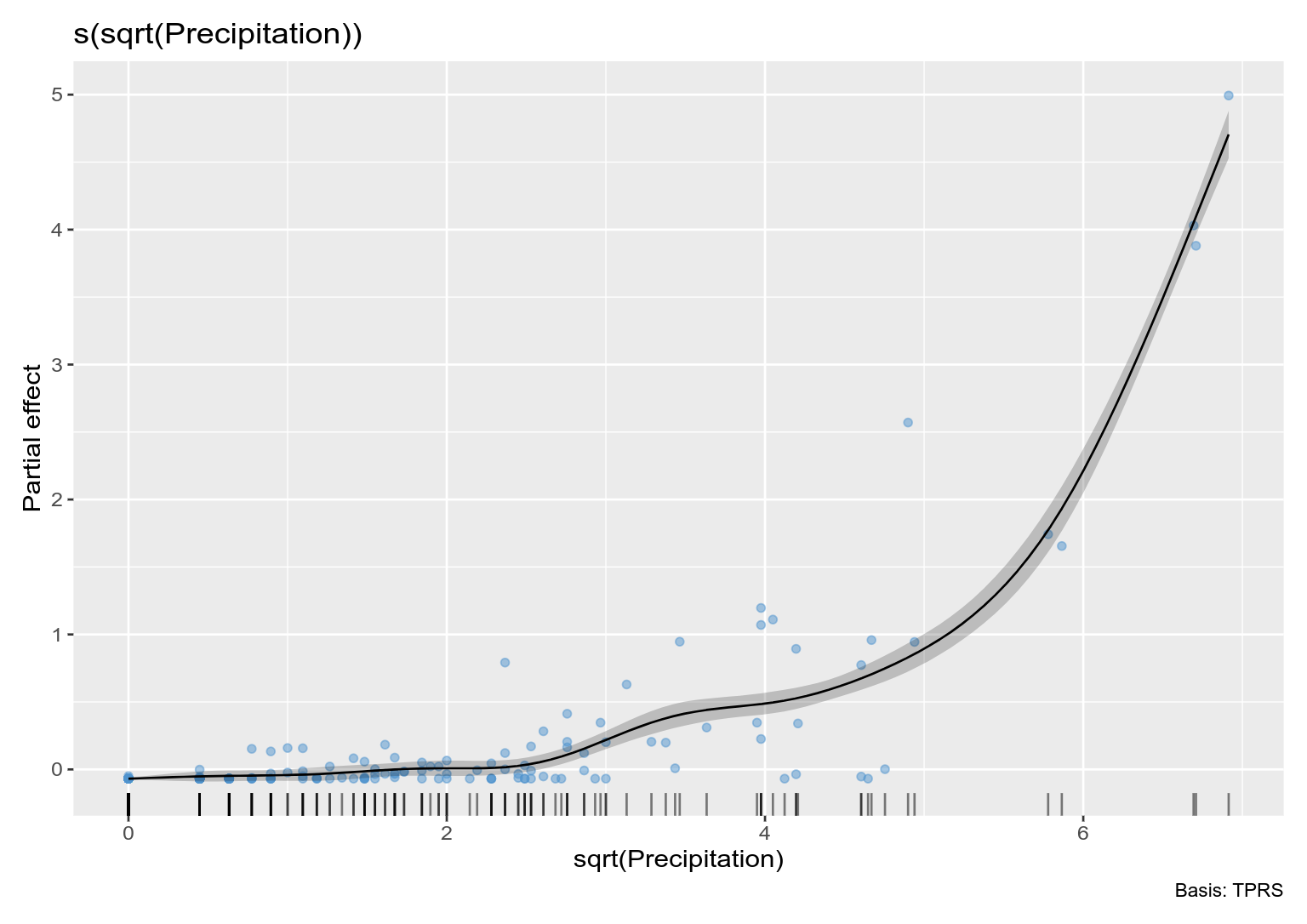
Note that a few large values of Precipitation are driving the wiggles in the function. We really need to spread these out. One way is to square root transform the values (you have 0s so a log transform is out of the question - more on this later). Below I repeat the above steps on square root transformed data:
m_orig_sqrt <- gam(DailyIncrease ~ s(sqrt(Precipitation)),
    data = pre, method = "REML")
summary(m_orig_sqrt)
> summary(m_orig_sqrt)

Family: gaussian
Link function: identity

Formula:
DailyIncrease ~ s(sqrt(Precipitation))

Parametric coefficients:
            Estimate Std. Error t value Pr(>|t|)
(Intercept)  0.06864    0.00559   12.28   <2e-16 ***
---
Signif. codes:  0 ‘***’ 0.001 ‘**’ 0.01 ‘*’ 0.05 ‘.’ 0.1 ‘ ’ 1

Approximate significance of smooth terms:
                         edf Ref.df     F p-value
s(sqrt(Precipitation)) 8.287  8.849 474.6  <2e-16 ***
---
Signif. codes:  0 ‘***’ 0.001 ‘**’ 0.01 ‘*’ 0.05 ‘.’ 0.1 ‘ ’ 1

R-sq.(adj) =  0.885   Deviance explained = 88.7%
-REML = -313.63  Scale est. = 0.01706   n = 546
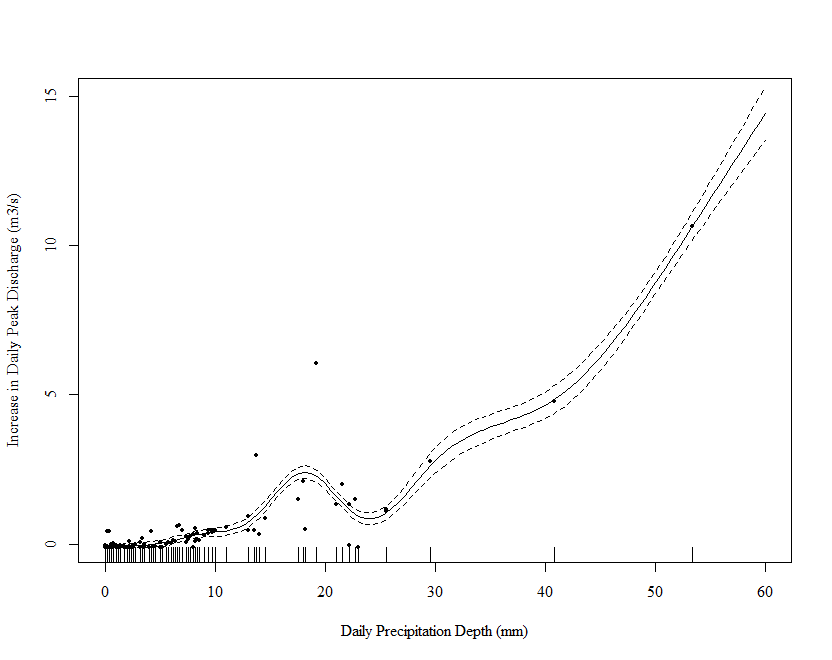
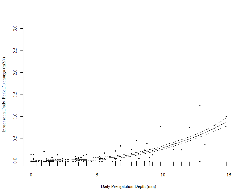
# plot
draw(m_orig_sqrt, residuals = TRUE)
This is better but not perfect. Note however that the excessive wiggliness in the estimated function has been removed.
Models for both data sets
Here I show three different ways to model both of the data sets in one model.
Start by combining the data into a single data frame
# combine into a single data set with a prepost variable coding for the data set
# I also square root transform precip here to avoid doing it in the model
combined <- pre |>
    bind_rows(post) |>
    mutate(prepost = rep(c("pre", "post"), times = c(nrow(pre), nrow(post))),
        prepost = factor(prepost, levels = c("pre", "post")),
    root_precip = sqrt(Precipitation))
Factor by smooths
First the factor by model. Note that we need to include the by factor as a parametric term to model the group means.
# fit the factor by model
m_f_by <- gam(DailyIncrease ~ prepost + s(root_precip, by = prepost),
    data = combined, method = "REML")
This model has fitted two separate smooths, one per data set, as shown in the model output:
> summary(m_f_by)

Family: gaussian
Link function: identity

Formula:
DailyIncrease ~ prepost + s(root_precip, by = prepost)

Parametric coefficients:
            Estimate Std. Error t value Pr(>|t|)
(Intercept) 0.063371   0.008359   7.581 7.36e-14 ***
prepostpost 0.052715   0.011808   4.464 8.88e-06 ***
---
Signif. codes:  0 ‘***’ 0.001 ‘**’ 0.01 ‘*’ 0.05 ‘.’ 0.1 ‘ ’ 1

Approximate significance of smooth terms:
                             edf Ref.df     F p-value
s(root_precip):prepostpre  7.847  8.441 224.0  <2e-16 ***
s(root_precip):prepostpost 8.672  8.957 548.6  <2e-16 ***
---
Signif. codes:  0 ‘***’ 0.001 ‘**’ 0.01 ‘*’ 0.05 ‘.’ 0.1 ‘ ’ 1

R-sq.(adj) =  0.862   Deviance explained = 86.4%
-REML = -190.21  Scale est. = 0.037884  n = 1095
The two lines for the smooth terms are separate tests of \text{H}_0: f(x_i) = 0 \; \forall \; i.
The two fitted smooths are visualised using
draw(m_f_by, grouped_by = TRUE)
As such there is nothing in this model that shows the difference between the two smooths. We can, however, compute this difference because we fitted both smooths in a single model:
difference_smooths(m_f_by, smooth = "s(root_precip)") |>
    draw()
This is showing that the pre smooth is lower than the "post" smooth around 4 root precip and at large values of root precip. It's not too difficult to plot this on the not-square-root scale but I won't show that as this is long enough already.
Ordered factor by smooths
Another option that does include an estimate of the difference is to set the model up using and ordered factor. In this model we fit a reference smooth and then smooth differences for the other levels. First we need to form the ordered factor and set the contrasts on this term to the usual treatment contrasts for easier interpretation
# next we fit the ordered factor version. Here I have said that `pre` is the
# reference level, which is important
combined <- combined |>
    mutate(prepost_o = ordered(prepost, levels = c("pre", "post")))
# set the contrasts to the usual treatment one
contrasts(combined$prepost_o) <- "contr.treatment"
Then we fit the model
m_ord_by <- gam(DailyIncrease ~ prepost_o +
        s(root_precip) + s(root_precip, by = prepost_o),
    data = combined, method = "REML")
summary(m_ord_by)
> summary(m_ord_by)

Family: gaussian
Link function: identity

Formula:
DailyIncrease ~ prepost_o + s(root_precip) + s(root_precip, by = prepost_o)

Parametric coefficients:
              Estimate Std. Error t value Pr(>|t|)
(Intercept)   0.062932   0.008373   7.516 1.18e-13 ***
prepost_opost 0.052965   0.011832   4.476 8.41e-06 ***
---
Signif. codes:  0 ‘***’ 0.001 ‘**’ 0.01 ‘*’ 0.05 ‘.’ 0.1 ‘ ’ 1

Approximate significance of smooth terms:
                               edf Ref.df      F p-value
s(root_precip)               7.627  8.267 230.61  <2e-16 ***
s(root_precip):prepost_opost 8.318  8.751  59.89  <2e-16 ***
---
Signif. codes:  0 ‘***’ 0.001 ‘**’ 0.01 ‘*’ 0.05 ‘.’ 0.1 ‘ ’ 1

R-sq.(adj) =  0.861   Deviance explained = 86.3%
-REML = -191.1  Scale est. = 0.038043  n = 1095
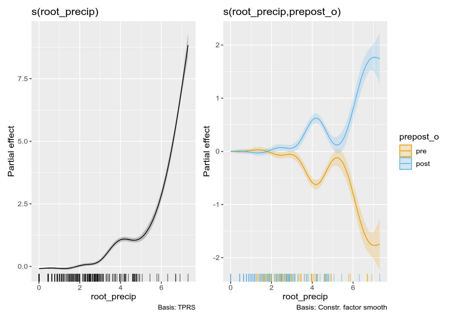
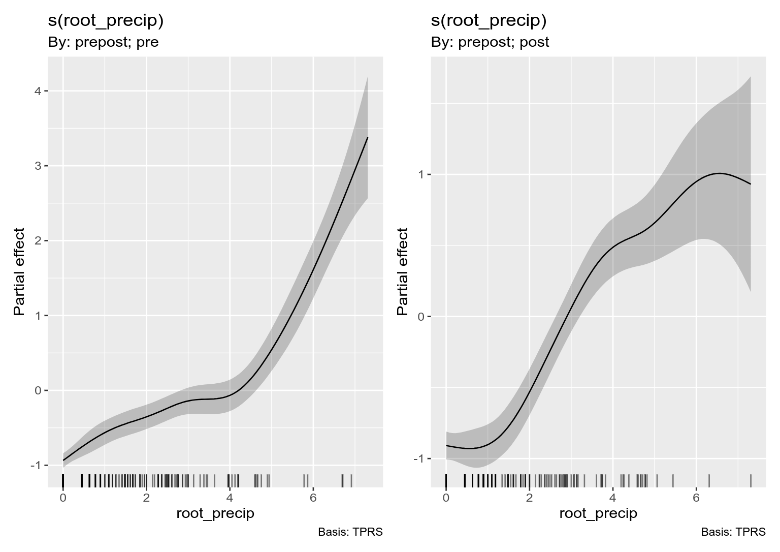
and visualise it using
draw(m_ord_by)
The second plot shown is how the smooth of root_precip for the "post" group differs from the reference smooth (for the "pre" group); again we see the tendency for the "post" group to be larger than the pre group.
Constrained factor smooths
Another option is the constrained factor smooth basis "sz". This basis allows us to fit a GAM with a "main effect" smooth and then difference smooths for the levels of a factor, which show how each level differs from the average or "main effect" smooth.
m_sz <- gam(DailyIncrease ~ s(root_precip) +
        s(root_precip, prepost_o, bs = "sz"),
    data = combined, method = "REML")

# model summary
summary(m_sz)
Note that
- in this model we do not need the parametric factor term (the group means are included in the
sz basis
- we set the special basis using the
bs argument
- the first smooth in the model is the average or "main effect" smooth
- the second smooth represents two smooth differences from this average smooth, one per level of the factor.
The fitted model is plotted using
draw(m_sz)
Here, the second plot looks weird because you only have a two levels, so they are mirror images of one another.
Two separate models
If all you want to do is compare smooths, then you can do it visually with gratia::compare_smooths():
m_pre <- gam(DailyIncrease ~ s(root_precip),
    data = combined |> filter(prepost == "pre"), method = "REML")
m_post <- gam(DailyIncrease ~ s(root_precip),
    data = combined |> filter(prepost == "post"), method = "REML")

compare_smooths(m_pre, m_post) |>
    draw()
…but not so fast
The above walk through and your approach in general is ignoring some pretty important features of your data which you need to account for.
Issues
The main issues with your approach are:
-
you're ignoring the time aspect - these data are collected in time order, and are thus not independent. All the intervals around the functions shown in the above figures are simply wrong - to narrow - because they assumed that the data were, conditional upon the model, independent.
-
as you currently have it, your response can't be lower than zero. You are truncating the data at 0 because a negative increase is a decrease. Such data can't be Gaussian, which allows for negative values. You can see the problems this causes in some of the figures, where the estimated smooth goes negative. You would need to fit a model that doesn't admit negative values, such as the Tweedie:
 m_tw_f_by <- gam(DailyIncrease ~ prepost + s(root_precip, by = prepost),
     data = combined, method = "REML", family = tw())
But that also doesn't account for the first problem.
It seems like you are causing more problems for yourself by processing the data two early. Why not model the discharge itself as a function of time and include the instantaneous effect of precipitation? You might get more specific help if you spell out what you are trying to do in general rather than tackle this one specific aspect.
But, for example:
combined <- combined |>
    mutate(year = format(Date, "%Y") |> as.numeric(),
        fyear = factor(year),
        doy = format(Date, "%j") |> as.numeric())

m_time <- bam(Discharge ~ prepost +   # treatment effect
        s(fyear, bs = "re") +         # random year effect
        s(doy, by = fyear, k = 100) + # smooth of time within year
        s(root_precip, by = prepost), # smooth effect of precip
    data = combined,
    method = "fREML",
    family = tw(link = "log"),
    discrete = TRUE, nthreads = 3)
You have one observation with 0 discharge observed which seems unlikely?
> combined |> filter(!Discharge > 0)
# A tibble: 1 × 11
  Date       Discharge Precipitation DailyChange DailyIncrease prepost root_precip prepost_o  year
  <date>         <dbl>         <dbl>       <dbl>         <dbl> <fct>         <dbl> <ord>     <dbl>
1 2012-05-28         0            17        5.56             0 pre            4.12 pre        2012
# ℹ 2 more variables: fyear <fct>, doy <dbl>
Hence the Tweedie, which allows 0s.
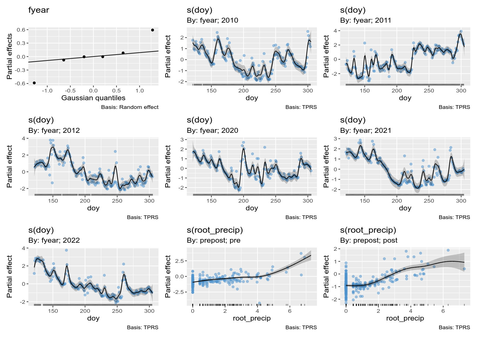
This estimated smooths are:
You can then estimate quantities of interest from that model, such as what is the effect on the discharge of precipitation in the two settings?
This is just for illustration; you'd want to check lots of assumptions here, and there may well still be unmodelled autocorrelation for example.
What I have done in this model is estimate the raw discharge values as a function of:
- the day of year within year -
s(doy, by = fyear, k = 100) to account for the different discharge patterns within each year that you observed. k is set large to allow for the rapid changes and peaks in discharge,
- the year of observation -
s(fyear, bs = "re") which is a random intercept for year as with the big gap it seems unreasonable to model these are a single time series,
- the effects of precipitation on discharge -
s(root_precip, by = prepost) which is allowed to vary between the two periods,
- the treatment mean effects -
prepost
As this model is getting a bit large I turned on some tricks to model this using a fast-fitting approach using multiple CPU cores. Note the use of bam() over gam(), discrete = TRUE, method = "fREML", and nthreads = 3..
To test if the slopes of the two precip curves differ, you could compute the derivatives of those two smooths using gratia::derivatives(). This would be the derivative on the log scale however. To get this value on the response scale we'd need to use posterior simulation via fitted_samples() or possibly the new function response_derivatives(). The former would allow you to estimate a difference of derivatives but you'd need to compute the derivatives (using finite differences) yourself for each draw from the posterior. It's not hard to do this, once you know the recipe.
The latter, response_derivatives() would compute the derivatives on the response scale. For this you need the development version of gratia:
discharge_d <- response_derivatives(m_time, focal = "root_precip",
    data = ds, n_sim = 10000, seed = 10,
    exclude = sms[c(1:7)])

discharge_d
> discharge_d
# A tibble: 200 × 9
    .row .focal      .derivative .lower_ci .upper_ci prepost fyear   doy root_precip
   <int> <chr>             <dbl>     <dbl>     <dbl> <fct>   <fct> <dbl>       <dbl>
 1     1 root_precip     0.0613     0.0179    0.131  pre     2020    213      0
 2     2 root_precip    -0.0124    -0.0785    0.0467 post    2020    213      0
 3     3 root_precip     0.0630     0.0186    0.135  pre     2020    213      0.0738
 4     4 root_precip    -0.0118    -0.0752    0.0467 post    2020    213      0.0738
 5     5 root_precip     0.0646     0.0200    0.139  pre     2020    213      0.148
 6     6 root_precip    -0.0108    -0.0706    0.0460 post    2020    213      0.148
 7     7 root_precip     0.0660     0.0218    0.142  pre     2020    213      0.221
 8     8 root_precip    -0.00942   -0.0649    0.0451 post    2020    213      0.221
 9     9 root_precip     0.0672     0.0239    0.144  pre     2020    213      0.295
10    10 root_precip    -0.00759   -0.0583    0.0433 post    2020    213      0.295
# ℹ 190 more rows
# ℹ Use `print(n = ...)` to see more rows
and then plot
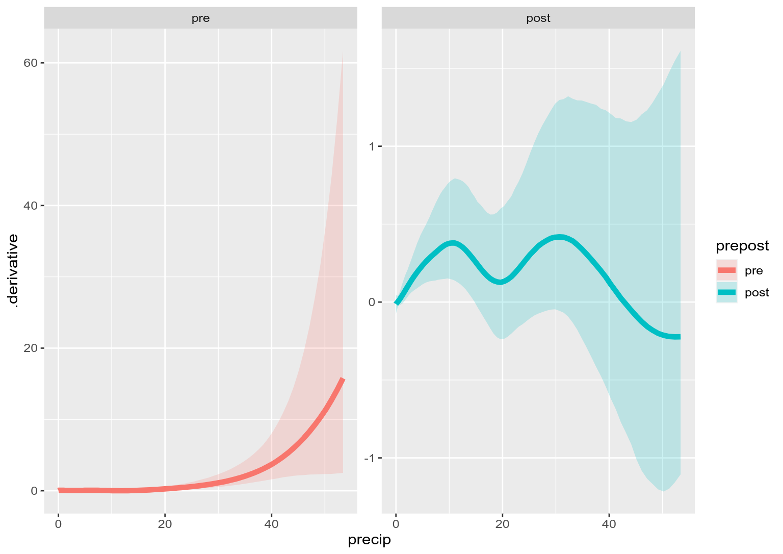
discharge_d |>
    mutate(precip = root_precip^2) |>
    ggplot(aes(x = precip, y = .derivative, group = prepost)) +
    geom_ribbon(aes(ymin = .lower_ci, ymax = .upper_ci, fill = prepost),
        alpha = 0.2) +
    geom_line(aes(colour = prepost), linewidth = 2) +
    facet_wrap(~ prepost, scales = "free_y")
which is consistent with the estimated smooths:
Note the derivative is positive in the post setting, except for the precip > 40 (root_precip > ~6.3), which could be fixed a little by reducing k to be lower than the default to allow less wiggliness.
The above is just for illustration; a proper analysis would need to delve in the modelling more.