I had to alter what you provided so as to be runnable.
library(tidyverse)
library(metan)

R <- readr::read_delim("Treat Year Rep GY OC N P K S Zn Cu
Control 2007 1 1.82 8.20 0.90 5.00 0.09 4.50 2.00 4.60
Control 2007 2 1.84 10.50 0.70 6.00 0.07 6.00 1.30 3.60
Control 2007 3 1.79 9.20 1.10 4.00 0.11 3.30 1.50 5.00
Rev.control 2007 1 10.57 12.30 1.20 11.00 0.13 5.10 5.50 5.60
Rev.control 2007 2 10.60 14.20 1.40 14.00 0.15 6.00 6.30 3.90
Rev.control 2007 3 10.63 10.40 1.00 17.00 0.11 4.50 4.10 7.00
NPK 2007 1 9.92 11.60 1.10 24.00 0.10 6.10 2.60 5.50
NPK 2007 2 9.93 10.00 0.90 21.00 0.15 7.10 1.80 6.00
NPK 2007 3 9.93 10.80 1.30 24.00 0.19 5.10 3.40 4.10
NPKS 2007 1 10.56 13.00 1.30 14.00 0.10 7.00 5.20 5.60
NPKS 2007 2 10.62 13.60 1.40 12.00 0.14 4.10 6.50 6.00
NPKS 2007 3 10.44 12.70 1.20 16.00 0.12 5.10 3.90 4.90
NPKSZn 2007 1 10.77 16.00 1.50 28.00 0.11 9.00 3.60 5.60
NPKSZn 2007 2 10.73 15.00 1.40 30.00 0.14 11.00 2.50 6.00
NPKSZn 2007 3 10.81 14.00 1.60 26.00 0.11 7.00 4.70 5.50
NPKSZnCu 2007 1 11.56 14.00 1.20 20.00 0.16 8.50 4.00 9.60
NPKSZnCu 2007 2 11.46 13.20 1.40 22.00 0.14 10.00 3.00 7.60
NPKSZnCu 2007 3 11.65 14.50 1.60 24.00 0.12 7.00 4.70 11.00
Control 2017 1 3.36 12.87 1.05 5.81 0.08 10.13 3.06 0.58
Control 2017 2 3.53 12.48 1.33 7.61 0.08 10.44 2.91 0.60
Control 2017 3 3.45 12.87 1.05 8.08 0.08 11.45 2.70 0.60
Rev.control 2017 1 11.99 14.43 1.61 17.20 0.13 14.45 4.18 1.15
Rev.control 2017 2 11.33 14.82 1.68 15.95 0.14 16.15 4.31 1.13
Rev.control 2017 3 12.14 15.60 1.54 15.00 0.10 19.41 4.25 1.20
NPK 2017 1 11.91 18.72 1.96 23.45 0.09 10.21 4.01 0.53
NPK 2017 2 11.12 19.11 1.82 23.36 0.13 10.20 4.43 0.53
NPK 2017 3 11.74 19.50 2.03 23.72 0.09 11.44 4.27 0.53
NPKS 2017 1 11.48 20.67 2.10 23.90 0.10 15.26 6.22 0.55
NPKS 2017 2 11.16 20.67 2.03 22.40 0.13 14.91 5.94 0.55
NPKS 2017 3 12.05 20.67 2.38 24.50 0.13 14.37 6.26 0.55
NPKSZn 2017 1 12.42 20.28 1.82 29.72 0.13 19.52 10.90 0.60
NPKSZn 2017 2 12.06 19.89 2.24 23.86 0.12 16.31 9.88 0.58
NPKSZn 2017 3 12.62 20.28 2.10 20.44 0.13 17.63 11.13 0.55
NPKSZnCu 2017 1 12.61 19.50 2.17 25.61 0.12 17.52 11.74 1.43
NPKSZnCu 2017 2 12.44 19.11 2.38 27.20 0.12 15.89 11.15 1.40
NPKSZnCu 2017 3 12.39 20.67 2.03 25.99 0.14 17.93 11.76 1.48",delim=" ")


CM<-corr_coef(R[4:11])
CM

P<-plot(CM,reorder = FALSE, digits.cor = 3)+
  theme(axis.text.x = element_text(color = "black",size = 10, face = "bold"))+
  theme(axis.text.y = element_text(color = "black",size = 10, face = "bold"))+
  theme(plot.margin = margin(0.6,0.6,0.6,0.6, "cm"))+
  scale_fill_gradient2(low = "#6D9EC1", mid = "white", high ="#E46726", midpoint = 0,
                       limits = c(-1,1), space = "Lab",
                       name="Pearson\nCorrelation")

P
this produced
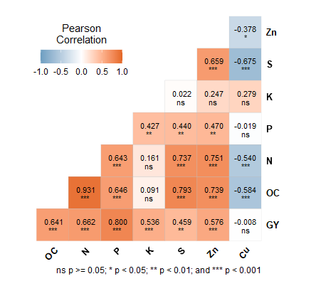
wherein it seems to me that following your use of digits.cor = 3, there are precisely 3 values after each decimal point within the cells. for example on row P; 0.440 is the second value.