I'm trying to replicate some analysis where the terms x and y are related using the following mathematical equation, where A through G are dimensionless constants:
y = \frac{Ax^2+Bx+C+Dx^{-1}}{Ex^2+Fx+Gx}
I am at a complete loss as to how to turn a tibble (for sake of simplicity, say it is named df and the columns are just x and y) into a model that follows this equation. Is this an nlm() job?
This is something I struggle with; transforming a known mathematical expression into the R formula that could produce it. For full context, this is a model taken from an Excel spreadsheet where A through G were given and you just had to plug in your value of x. I have my own data that I'd like to use to recreate the same kind of x-y curve.
This doesnt seem workable on its face...
Fx and Gx are both there. thats an infinity of solutions even for fixed known x/y pairs...
maybe it should be only Fx and forget the Gx, as the x is the same power ?
I think this requires a nonlinear optimization with optim.
You must write a function that accepts as an argument the parameter values A, B, C, ... and returns a sum of square error.
Then ask optim to adjust the parameter values to minimize the error.
In my experience you have to be careful that the arguments are consistent between all your functions. You'll have a function for the model, a function that returns the error, and optim, that requires the arguments to be specified a certain way.
Here's my solution adapted from work I've done in the past. method = "BFGS" generally works best for me.
library(tidyverse)
# model
my_model <- function(p, x) {
y <- p["A"] * x^2 + p["B"] * x + p["C"] + p["D"] / x # just the numerator
return(y)
}
# real values
p <- c(A = 1, B = 2, C = 3, D = 4)
# simulated data
# make x order 1 otherwise some model terms will dominate
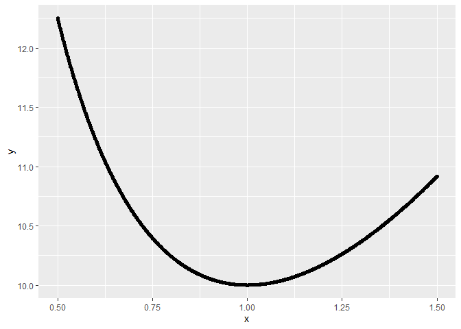
my_data <- tibble(
x = seq(0.5, 1.5, .001),
y = my_model(p, x) # + 0.01 + runif(length(x))
)
with(my_data, qplot(x, y))
# objective fn
calc_obj <- function(p, model, df) {
  resid <- model(p, df$x) - df$y
  return(sqrt(sum(resid^2)))
}

# initial guess
p0 <- c(A = 1.1, B = 2.2, C = 3.3, D = 4.4)

# try to recover the real values through nonlinear opt
soln <- optim(
  par = p0,
  fn = calc_obj,
  method = "BFGS",
  control = list(trace = 5, REPORT = TRUE),
  model = my_model,
  df = my_data
)
#> initial  value 33.193450
#> iter   2 value 5.247466
#> iter   3 value 4.227183
#> iter   4 value 1.328340
#> iter   5 value 0.789765
#> iter   6 value 0.344899
#> iter   7 value 0.155544
#> iter   8 value 0.109454
#> iter   9 value 0.084487
#> iter  10 value 0.040555
#> iter  11 value 0.035276
#> iter  12 value 0.017175
#> iter  13 value 0.007212
#> iter  14 value 0.006679
#> iter  15 value 0.006320
#> iter  16 value 0.005695
#> iter  17 value 0.005051
#> iter  17 value 0.005051
#> iter  18 value 0.004443
#> iter  19 value 0.004018
#> iter  20 value 0.002721
#> iter  21 value 0.002691
#> iter  21 value 0.002691
#> iter  22 value 0.002289
#> iter  23 value 0.002194
#> iter  24 value 0.001797
#> iter  24 value 0.001797
#> iter  25 value 0.001328
#> iter  26 value 0.001268
#> iter  27 value 0.001174
#> iter  28 value 0.001153
#> iter  29 value 0.001147
#> iter  30 value 0.001145
#> iter  31 value 0.001145
#> iter  32 value 0.001145
#> iter  33 value 0.001145
#> iter  34 value 0.000906
#> iter  35 value 0.000877
#> iter  35 value 0.000877
#> iter  36 value 0.000766
#> iter  37 value 0.000746
#> iter  38 value 0.000688
#> iter  38 value 0.000688
#> iter  39 value 0.000637
#> iter  40 value 0.000637
#> iter  40 value 0.000637
#> iter  41 value 0.000615
#> iter  42 value 0.000615
#> iter  43 value 0.000598
#> iter  44 value 0.000598
#> iter  45 value 0.000597
#> iter  45 value 0.000597
#> iter  46 value 0.000591
#> iter  47 value 0.000585
#> iter  48 value 0.000580
#> iter  49 value 0.000577
#> iter  49 value 0.000577
#> iter  50 value 0.000574
#> iter  51 value 0.000569
#> iter  52 value 0.000569
#> iter  53 value 0.000569
#> iter  53 value 0.000569
#> iter  54 value 0.000566
#> iter  55 value 0.000563
#> iter  56 value 0.000546
#> iter  57 value 0.000546
#> iter  58 value 0.000546
#> iter  58 value 0.000546
#> iter  59 value 0.000540
#> iter  60 value 0.000537
#> iter  61 value 0.000534
#> iter  62 value 0.000533
#> iter  62 value 0.000533
#> iter  63 value 0.000511
#> iter  64 value 0.000511
#> iter  65 value 0.000510
#> iter  66 value 0.000509
#> iter  67 value 0.000509
#> iter  68 value 0.000509
#> iter  69 value 0.000509
#> iter  69 value 0.000509
#> iter  70 value 0.000507
#> iter  71 value 0.000503
#> iter  72 value 0.000502
#> iter  73 value 0.000502
#> iter  74 value 0.000502
#> iter  75 value 0.000502
#> iter  76 value 0.000502
#> iter  76 value 0.000502
#> iter  77 value 0.000496
#> iter  78 value 0.000496
#> iter  79 value 0.000492
#> iter  79 value 0.000492
#> iter  80 value 0.000488
#> iter  81 value 0.000481
#> iter  82 value 0.000479
#> iter  83 value 0.000476
#> iter  84 value 0.000475
#> iter  84 value 0.000475
#> iter  85 value 0.000472
#> iter  86 value 0.000468
#> iter  87 value 0.000468
#> iter  88 value 0.000467
#> iter  88 value 0.000467
#> iter  89 value 0.000458
#> iter  90 value 0.000449
#> iter  91 value 0.000443
#> iter  92 value 0.000436
#> iter  92 value 0.000436
#> iter  93 value 0.000434
#> iter  94 value 0.000430
#> iter  95 value 0.000424
#> iter  96 value 0.000424
#> iter  96 value 0.000424
#> iter  97 value 0.000421
#> iter  98 value 0.000416
#> iter  99 value 0.000415
#> iter 100 value 0.000413
#> final  value 0.000413
#> stopped after 100 iterations

# results
tibble(
  name       = names(p),
  true_value = p,
  guess      = p0,
  solution   = soln$par
) %>%
  print()
#> # A tibble: 4 x 4
#>   name  true_value guess solution
#>   <chr>      <dbl> <dbl>    <dbl>
#> 1 A              1   1.1    0.999
#> 2 B              2   2.2    2.00
#> 3 C              3   3.3    3.00
#> 4 D              4   4.4    4.00
I'm interested as well now to see indeed if there is a way to do this with the provided formula. I tried to use nls() but I keep getting the error :
data = data.frame(x = 10:1, y = 1:10)
nls(y ~ (Aa*x^2 + Bb*x + Cc + Dd*x^(-1)) * Ee,
    data, start = list(Aa = 1, Bb = 1, Cc = 1, Dd = 1, Ee = 1))

Error in nlsModel(formula, mf, start, wts, scaleOffset = scOff, nDcentral = nDcntr) :
  singular gradient matrix at initial parameter estimates
As @nirgrahamuk showed, this might be because of the formula, and I like his approach for the estimation of the initial values. I'm not good at this type of maths, so will follow closely to see which approach works best in the end
Oh. I think in the data you created for the example y = 1/x. So you should get As=Bb=Cc=0. But then Dd and Ee are interchangeable. That's probably the source of the error.
This is not the kind of problem that one typically encounters in applied statistics. You know the data generation process in functional form but not the coefficients. Think of someone telling you "I know that the circumference of a circle is related to the radius but I don't know what the constant is". How would you find PI? But this relationship has many more degrees of freedom.
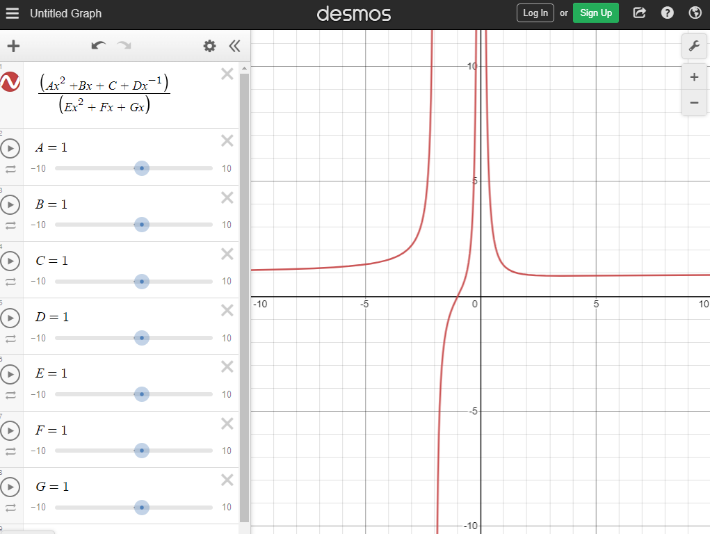
So if we plug in your original equation to something like Desmos, we can see that if all the parameters = 1, we get really interesting plot with lines going down each axis.
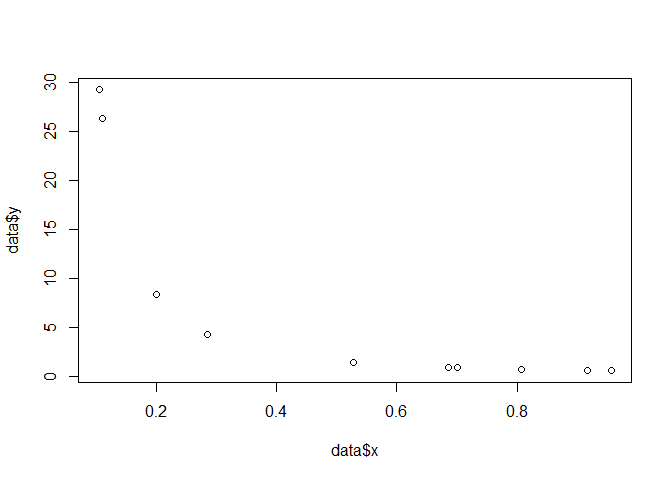
If you make a scatter plot of your XY data, you could use Desmos by adjusting the sliders until you get something that you could imagine would fit your data. Then use those values as starting values in nls().
I guess my concern is what sort of data would you have that requires such a function? You have negative X and Y values too? Are you only concerned with what is going on when X and Y are both positive?
I agree with @arthur.t in that your goal to come up with the parameter values will require some clever work with nls and optim. This is one reason why self-starting functions are popular (some included in stats and more available through other packages like nlraa.
Just as an example, here is a reprex that uses a self-starting function with 6 parameters. That is pretty close to your 7, and it demonstrates that your problem may be solved somehow.
library(tidyverse)
library(nlraa)
library(minpack.lm)

fit <- minpack.lm::nlsLM(
    Petal.Width ~ SSsharp(Sepal.Length, a, b, c, d, e, f), data = iris
    )

fit

iris %>%
    ggplot(aes(Sepal.Length, Petal.Width)) +
    geom_point() +
    geom_line(aes(y = predict(fit))) +
    # or
    geom_line(stat = "smooth",
              method = "nlsLM",
              formula = y ~ SSsharp(x, a, b, c, d, e, f),
              se = FALSE,
              color = "red")
If the equation is something that an engineer came up with in Excel solver, frankly you may want to scrap it and start fresh. I've seen some terrible models created by people who didn't understand overfitting.
The practice of "curve fitting" with polynomials and Excel solver is best left in the past.

 Then again I was doing this totally at random ...