Extract time then save into a new dataframe

Please can someone advise where i am going wrong. I have the code below to extract hour, minutes, and seconds. It doesn't work. I am getting an error message: Error in UseMethod("mutate_") :
no applicable method for 'mutate_' applied to an object of class "function"

lubridate::ymd_hms(as.character(d1$timestamp, tz = "UTC"))

df %>% mutate(hours=hour(strptime(d1$timestamp, %H:%M')) %>% as.character() )

I'm not sure if I understand the logic behind your code but, you can try something like this

library(dplyr)
library(lubridate)

df <- tibble(timestamp = ymd_hms('2019-01-04 10:24:20', '2019-01-04 10:25:10'))
df %>% 
    mutate(hours=hour(timestamp), minutes = minute(timestamp), seconds = second(timestamp))
#> # A tibble: 2 x 4
#>   timestamp           hours minutes seconds
#>   <dttm>              <int>   <int>   <dbl>
#> 1 2019-01-04 10:24:20    10      24      20
#> 2 2019-01-04 10:25:10    10      25      10

Created on 2019-01-04 by the reprex package (v0.2.1)

1 Like

Thanks for your help. Is it possible to meger hour, minute and seconds as one column? Also what is the correct data format for the field? should it be integer? As i am trying to plot this data into a graph.

Would this work for you?

library('tidyverse')
library('lubridate')
df = tibble(timestamp = ymd_hms('2019-01-04 10:24:20', '2019-01-04 10:25:10'))
df %>% mutate(clock = timestamp %>% str_split(' ') %>% map_chr(2) %>% hms)
# A tibble: 2 x 2
  timestamp           clock       
  <dttm>              <S4: Period>
1 2019-01-04 10:24:20 10H 24M 20S 
2 2019-01-04 10:25:10 10H 25M 10S 

Hope it helps :slightly_smiling_face:
Leon

I you just want to use time on a continuous scale there is no need to modify your timestamp, you can use scale_x_datetime()

library(ggplot2)
library(dplyr)
data <- data.frame(
    time = as.POSIXct(c("2018-11-06 08:00:33", "2018-11-06 09:00:35",
                        "2018-11-06 10:00:35", "2018-11-06 11:00:33",
                        "2018-11-06 12:00:41", "2018-11-06 13:00:34", "2018-11-06 14:00:38",
                        "2018-11-06 15:00:37", "2018-11-06 16:00:34", "2018-11-06 17:00:34",
                        "2018-11-06 18:00:37", "2018-11-06 19:00:33", "2018-11-06 20:00:36",
                        "2018-11-06 21:00:35", "2018-11-06 22:00:37",
                        "2018-11-06 23:00:36", "2018-11-07 00:00:35", "2018-11-07 01:00:34",
                        "2018-11-07 02:00:36", "2018-11-07 03:00:33", "2018-11-07 04:00:37")),
    ping = c(31.04, 30.09, 29.22, 29.33, 30.18, 27.8, 29.59, 29.87, 29.87,
             30.58, 32.2, 29.96, 31.84, 32.62, 30.98, 35.57, 32.41, 30.7,
             31.73, 29.21, 32.33)
)

data %>% 
    ggplot(aes(x = time, y = ping)) +
    geom_line() +
    scale_x_datetime(date_breaks = "1 hour", date_labels = '%H:%M:%S') +
    theme(axis.text.x = element_text(angle=30, hjust=1, vjust = 1))
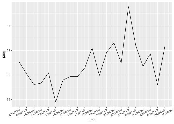
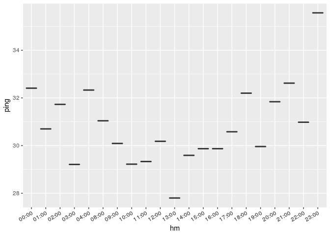
If you want to use time on a discrete scale you can do something like this

library(ggplot2)
library(dplyr)
library(tibbletime)

data <- data.frame(
    time = as.POSIXct(c("2018-11-06 08:00:33", "2018-11-06 09:00:35",
                        "2018-11-06 10:00:35", "2018-11-06 11:00:33",
                        "2018-11-06 12:00:41", "2018-11-06 13:00:34", "2018-11-06 14:00:38",
                        "2018-11-06 15:00:37", "2018-11-06 16:00:34", "2018-11-06 17:00:34",
                        "2018-11-06 18:00:37", "2018-11-06 19:00:33", "2018-11-06 20:00:36",
                        "2018-11-06 21:00:35", "2018-11-06 22:00:37",
                        "2018-11-06 23:00:36", "2018-11-07 00:00:35", "2018-11-07 01:00:34",
                        "2018-11-07 02:00:36", "2018-11-07 03:00:33", "2018-11-07 04:00:37")),
    ping = c(31.04, 30.09, 29.22, 29.33, 30.18, 27.8, 29.59, 29.87, 29.87,
             30.58, 32.2, 29.96, 31.84, 32.62, 30.98, 35.57, 32.41, 30.7,
             31.73, 29.21, 32.33)
)

data %>% 
    as_tbl_time(index = time) %>% 
    collapse_by('1 hour', side = 'start', clean = TRUE) %>%
    mutate(hm = format(time, "%H:%M")) %>% 
    ggplot(aes(x = hm, y = ping)) +
    geom_boxplot() +
    theme(axis.text.x = element_text(angle=30, hjust=1, vjust = 1))
3 Likes

Many Thanks for your help. I am trying to create a graph, which represent a timestamp and a variable of which it value is either on or off. The graph I am getting at the moment show two straight lines. Any idea why please?

Could you please turn this into a self-contained reprex (short for reproducible example)? It will help us help you if we can be sure we're all working with/looking at the same stuff.

install.packages("reprex")

If you've never heard of a reprex before, you might want to start by reading the tidyverse.org help page. The reprex dos and don'ts are also useful.

What to do if you run into clipboard problems

If you run into problems with access to your clipboard, you can specify an outfile for the reprex, and then copy and paste the contents into the forum.

reprex::reprex(input = "fruits_stringdist.R", outfile = "fruits_stringdist.md")

For pointers specific to the community site, check out the reprex FAQ.

1 Like

So, if you take a look at the reprex docs, you'll see you actually have to include the libraries and the data in the reprex itself (hence the self-contained). So, the errors you're getting here are just because the functions aren't available because the packages aren't attached.

Sorry, not sure how to include the data. Can you tell me which part in the repex doc cover this please?

Take a look at the post above by @andresrcs, specifically at the part where data object is created. This is one way to put your data in shareable form.

Another way is wrapr::draw_frame() (here is an example).

Finally, read following Do's and Don'ts on reprex page where first point (Use the smallest, simplest, most built-in data possible.) talks about how to share your data.

This topic was automatically closed 21 days after the last reply. New replies are no longer allowed.