Hey Flm and jrkrideau,
Thanks so much for your replies. I have made a bit more progress since my first post, but I am still not managing to succeed. I will post all code used in this latest method. For ease, I have reformatted the datetime column and have renamed columns to fit the tutorial I have been following.
Here is the data frame:
structure(list(Longitude = c(23.273798, 23.273798, 23.273798,
23.274721, 23.274721, 23.274721, 23.274818, 23.274818, 23.274818,
23.274818, 23.274818, 23.274818, 23.273766, 23.273766, 23.273766,
23.273766, 23.273787, 23.273766, 23.272833, 23.272833), Latitude = c(-34.035352,
-34.035352, -34.035352, -34.035388, -34.035388, -34.035388, -34.036117,
-34.036117, -34.036117, -34.036117, -34.036117, -34.036117, -34.038561,
-34.038561, -34.038561, -34.038561, -34.037691, -34.038561, -34.038562,
-34.038562), Time = structure(c(1583137800, 1583138100, 1583138400,
1583138700, 1583139000, 1583139300, 1583139600, 1583139900, 1583140200,
1583140500, 1583140800, 1583141100, 1583141400, 1583141700, 1583142000,
1583142300, 1583142600, 1583142900, 1583143200, 1583143500), class = c("POSIXct",
"POSIXt"), tzone = "UTC"), Herd = c("Pre", "Pre", "Pre", "Pre",
"Pre", "Pre", "Pre", "Pre", "Pre", "Pre", "Pre", "Pre", "Pre",
"Pre", "Pre", "Pre", "Pre", "Pre", "Pre", "Pre"), ID = 1:20,
X = c(19005904.835773, 19005904.835773, 19005904.835773,
19005851.64108, 19005851.64108, 19005851.64108, 19006097.6250832,
19006097.6250832, 19006097.6250832, 19006097.6250832, 19006097.6250832,
19006097.6250832, 19007020.3460048, 19007020.3460048, 19007020.3460048,
19007020.3460048, 19006717.0295294, 19007020.3460048, 19007087.0873124,
19007087.0873124), Y = c(10533131.9385612, 10533131.9385612,
10533131.9385612, 10533401.5758544, 10533401.5758544, 10533401.5758544,
10533491.9050809, 10533491.9050809, 10533491.9050809, 10533491.9050809,
10533491.9050809, 10533491.9050809, 10533396.998876, 10533396.998876,
10533396.998876, 10533396.998876, 10533328.6946106, 10533396.998876,
10533127.6196109, 10533127.6196109), Year = c(2020, 2020,
2020, 2020, 2020, 2020, 2020, 2020, 2020, 2020, 2020, 2020,
2020, 2020, 2020, 2020, 2020, 2020, 2020, 2020), DOY = c(62,
62, 62, 62, 62, 62, 62, 62, 62, 62, 62, 62, 62, 62, 62, 62,
62, 62, 62, 62)), projection = "+proj=utm +zone=11 +ellps=GRS80 +towgs84=0,0,0,0,0,0,0 +units=m +no_defs", row.names = c(NA,
20L), class = "data.frame")
The code I have used so far:
caribou.raw <- read.csv("./caribou.csv")
dim(caribou.raw)
names(caribou.raw)
head(caribou.raw)
str(caribou.raw)
caribou.raw$Herd<-as.factor(caribou.raw$Herd)
caribou.raw$Location.Date<-as.factor(caribou.raw$Location.Date)
caribou.raw$ID<-as.factor(caribou.raw$ID)
levels(caribou.raw$Herd)
caribou <- rename(caribou.raw, c(ID = "ID", Location.Date = "Time"))
table(caribou$Herd)
with(subset(caribou, Herd == "Pre"), plot(Longitude, Latitude, col = "blue"))
with(subset(caribou, Herd == "During"), points(Longitude, Latitude, col = "red"))
head(as.POSIXlt(caribou$Time, format = "%m/%d/%Y %H:%M", tz = "UTC"))
require(lubridate)
caribou$Time <- mdy_hm(caribou$Time)
last line fails to parse, but POSIX line seems to work.
range(caribou$Time) ## produces NAs
hour(caribou$Time)[1:10]
month(caribou$Time)[1:10]
yday(caribou$Time)[1:10]
caribou$Time[1:10]
diff(caribou$Time[1:10])
##to visualise
require(PBSmapping)
ll <- with(caribou, data.frame(X = Longitude, Y = Latitude))
attributes(ll)$projection <- "LL"
xy <- convUL(ll, km=TRUE)
caribou <- cbind(caribou, xy)
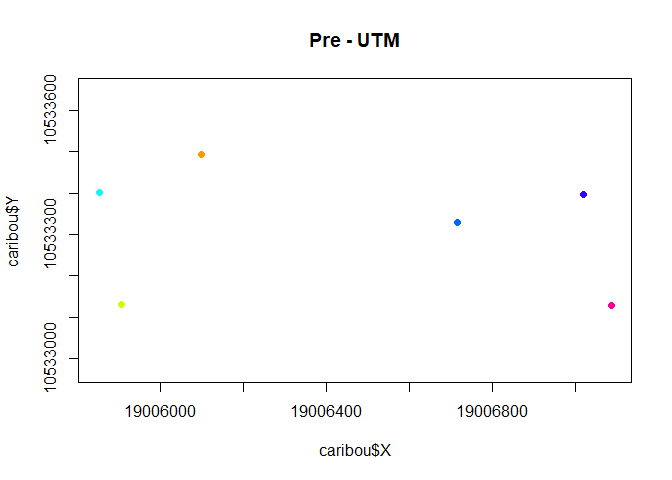
palette(rainbow(10))
with(subset(caribou, Herd == "Pre"),
plot(X,Y, asp=1, col = ID, pch = 19, cex= 0.5, main = "Pre - UTM"))
diff(range(xy$X))
diff(range(xy$Y))
ddply(caribou, "Herd", summarize,
n.loc = length(X),
n.ind = length(unique(ID)),
time.range = diff(range(Time)),
x.range.km = diff(range(X)), y.range.km = diff(range(Y)))
require(rgdal)
NWT.proj4 <- "+proj=lcc +lat_1=50 +lat_2=70 +lat_0=40 +lon_0=-96 +x_0=0 +y_0=0 +datum=NAD83 +units=m +no_defs"
XY <- project(cbind(caribou$Longitude, caribou$Latitude), NWT.proj4)
caribou$X <- XY[,1]
caribou$Y <- XY[,2]
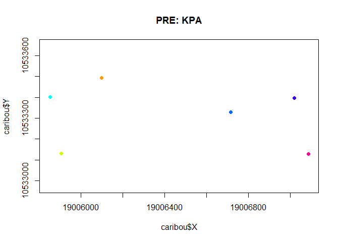
with(subset(caribou, Herd == "Pre"),
plot(X,Y, asp=1, col = ID, cex= 0.5, pch = 19,
main = "PRE: KPA"))
##produces NAs in seconds
ddply(caribou, "Herd", summarize, duration = diff(range(Time)))
#as a function
processCaribou <- function(caribou.raw, projection){
caribou <- rename(caribou.raw, c(ID = "ID", Location.Date = "Time"))
caribou$Time <- mdy_hm(caribou$Time)
caribou$X <- XY[,1]
caribou$Y <- XY[,2]
this line attached the projection as an "attribute" of the data
attributes(caribou) <- c(attributes(caribou), projection = projection)
return(caribou)
}
UTM11.proj <- "+proj=utm +zone=11 +ellps=GRS80 +towgs84=0,0,0,0,0,0,0 +units=m +no_defs"
caribou <- processCaribou(caribou.raw, UTM11.proj)
with(caribou,
plot(X/1000, Y/1000, col = alpha(as.integer(Herd), .2),
pch = 19, cex = 0.3, asp = 1, main = "All caribou"))
##produces error message: Warning message:
In alpha(as.integer(Herd), 0.2) : NAs introduced by coercion
##analysis part
caribou <- mutate(caribou, Year = year(Time), DOY = yday(Time))
caribou.daily <- ddply(caribou, c("ID", "Year", "DOY", "Herd", "ID"),
summarize, Latitude = mean(Latitude), Longitude = mean(Longitude), X = mean(X),
Y = mean(Y))
dim(caribou)
dim(caribou.daily)
head(caribou.daily)
caribou.daily <- mutate(caribou.daily, Date = ymd(paste(Year - 1, 12, 31)) +
ddays(DOY), Month = month(Date)) ##FAILS TO PARSE
attr(caribou.daily, "projection") <- attr(caribou, "projection")
pp5 <- subset(caribou.daily, Herd == "Pre")
Z <- pp5$X + (0+1i) * pp5$Y
StepLength <- Mod(diff(Z))
dT <- as.numeric(diff(pp5$Date))
table(dT)
Speed <- StepLength/dT
hist(Speed/1000, breaks = 50, col = "grey")
summary(Speed/1000) ## PRODUCES TABLE WITH “inf” and NAs
##none of the following works
computeDD <- function(data) {
Z <- data$X + (0+1i) * data$Y
StepLength <- c(NA, Mod(diff(Z)))
dT <- c(NA, as.numeric(diff(data$Date)))
Speed <- StepLength/dT
return(data.frame(data, StepLength, dT, Speed))
}
caribou.daily <- ddply(caribou.daily, "Herd", computeDD)
summary(caribou.daily)
boxplot((Speed/1000) ~ Month, data = subset(caribou.daily, Speed > 0), log = "y",
ylim = c(0.001, 100), ylab = "km/day", pch = 19, cex = 0.5, col = rgb(0,
Next I would like to calculate movement rates, home ranges and utilisation distributions, kernel density estimates, and eventually do mixed effects models between the three periods (pre, during, post), but I don't seem to get the data into the correct format to begin with, and then I get really lost making the rest of it work. I really really appreciate your advice. I'm sure there is a simpler way to do all of this to, but it is fairly new to me.
Thank you so much for your help!