Equality of marginal effects (first / second differences)

[scottcole2]

I want to test for statistical significance of an interaction between two categorical predictors (0 or 1) from a logit regression. (I have plotted predicted probabilities and see interesting dependencies, and now want to test for statistically different “marginal effects” (not model coefficients !)).

I define marginal effect as difference between two probabilities at the specific interacted values (both first and second differences).

My suggested approach and questions (see also reprex below):

1. Estimate Marginal Effects. First I must estimate two marginal effects (“first differences”). In my case: the effect of changes in SIZE at the two specific interacted values of LOC. Question: how to estimate these two specific marginal effects such that I can extract the variance estimates for (1) testing their equivalence (first diff) and (2) for use in the next step (second diff)? Packages like sjPlot provide pred probs, but don't do the simulation needed for estimating variances of effects; Packages like MARGINS/MFX/EFFECTS provide simulation, but can’t seem to be able to define the effects/1st diffs at the specific interacted values?

2. Statistical test. I want to use a Wald test to test equality of these two effects estimated above (i.e., a second difference). Ideally, I would extract relevant results from above as input to the Wald test (i.e., variance estimate of each marginal effect and the estimated covariance between the effects). Can somebody help here?

… or are there packages for testing significance of an interactions (second diff) that make this easier? Thanks in advance for help. See reprex with fake numbers below.

I’m basing my approach on Mize, T. D. (2019). Best Practices for Estimating, Interpreting, and Presenting Nonlinear Interaction Effects. Sociological Science, 6, 81–117. https://doi.org/10.15195/v6.a4

  suppressPackageStartupMessages({
    library(sjPlot)
    library(ggeffects)})
  
  # create ex. data set.  1 row per respondent (dataset shows 2 resp). 
  cedata.1 <- data.frame( id    =  c(1,1,1,1,1,1,2,2,2,2,2,2),    
                          QES    = c(1,1,2,2,3,3,1,1,2,2,3,3),   # Choice set   
                          Alt    = c(1,2,1,2,1,2,1,2,1,2,1,2),   # Alt 1 or Alt 2 in  choice set 
                          LOC    = c(0,0,1,1,0,1,0,1,1,0,0,1),   # attribute. binary categorical variable
                          SIZE   = c(1,1,1,0,0,1,0,0,1,1,0,1),   # attribute. binary categorical variable
                          Choice = c(0,1,1,0,1,0,0,1,0,1,0,1),   # if  Chosen (1) or not (0)
                          gender = c(1,1,1,1,1,1,0,0,0,0,0,0)   
  )
  
  # convert to factor as required by sjPlot
  cedata.1$Choice <- as.factor(cedata.1$Choice)
  cedata.1$LOC <- as.factor(cedata.1$LOC)
  cedata.1$SIZE <- as.factor(cedata.1$SIZE)
  
  # estimate model
glm.model <- glm(Choice ~  LOC*SIZE, data=cedata.1, family = binomial(link = "logit"))

  # estimate change in Pred Prob for the Interaction
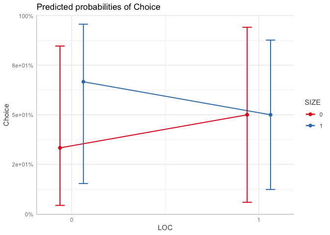
LOC.SIZE <- ggpredict(glm.model, terms = c("LOC", "SIZE")) 
LOC.SIZE
#> 
#> # Predicted probabilities of Choice
#> # x = LOC
#> 
#> # SIZE = 0
#> 
#> x | Predicted |   SE |       95% CI
#> -----------------------------------
#> 0 |      0.33 | 1.22 | [0.04, 0.85]
#> 1 |      0.50 | 1.41 | [0.06, 0.94]
#> 
#> # SIZE = 1
#> 
#> x | Predicted |   SE |       95% CI
#> -----------------------------------
#> 0 |      0.67 | 1.22 | [0.15, 0.96]
#> 1 |      0.50 | 1.00 | [0.12, 0.88]
#> Standard errors are on the link-scale (untransformed).

  # plot interaction
  plot(LOC.SIZE, connect.lines = TRUE)

  
  #  pander table for 1st / 2nd diff (thanks to @technocrat ... )
  # FUNCTIONS
  
  mk_2pl <- function(x) {
    prettyNum(x,digits = 2)
  }
  
  # CONSTANTS
  
  header_row  <- c("","Prob. of choosing",
                   "First Diff (Marg Eff)","Second Diff")
  col1  <- c("LOC=0:Size=0","LOC=0:SIZE=1","LOC=1:SIZE=0","LOC=1:SIZE=1")
  blank <- ""
  
  # ggpredict results extracted for formatting
  the_tests <- LOC.SIZE$predicted
  topfst <- LOC.SIZE$predicted[2]-LOC.SIZE$predicted[1]
  botfst <- LOC.SIZE$predicted[4]-LOC.SIZE$predicted[3]
  secdf  <- botfst - topfst
  
  # convert to strings
  col2 <- mk_2pl(the_tests)
  piece1 <- paste(mk_2pl(the_tests[2]),"-",mk_2pl(the_tests[1]),"=",mk_2pl(topfst))
  piece2 <- paste(mk_2pl(the_tests[4]),"-",mk_2pl(the_tests[3]),"=",mk_2pl(botfst))
  col4 <- paste(mk_2pl(botfst),"-",mk_2pl(topfst),"=",mk_2pl(secdf))
  col3 <- c(piece1,piece2)
  
  # create data frame
  
  assembled <- as.data.frame(cbind(col1,col2,col3,col4))
  colnames(assembled) <- header_row
  assembled[2,3] <- blank
  assembled[3,3] <- blank
  assembled[c(1,3,4),4] <- blank
  pander::pander(assembled)

	Prob. of choosing	First Diff (Marg Eff)	Second Diff
LOC=0:Size=0	0.33	0.67 - 0.33 = 0.33
LOC=0:SIZE=1	0.67		0 - 0.33 = -0.33
LOC=1:SIZE=0	0.5
LOC=1:SIZE=1	0.5	0.5 - 0.5 = 0