Dynamic Linear Model

[Desislava]

Hello everyone,

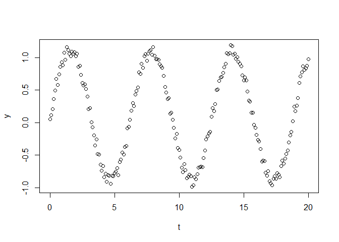
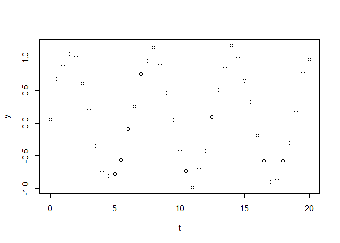
I am trying to do an interpolation of a high frequency data to low frequency. I tried with the dlm package but I cannot manage to obtain the unobserved monthly data. I have zero experience with state-space models and I would really appreciate if someone can advise what I am doing wrong and maybe recommend a suitable package if this is not the right one.

I attack the image so you can get an idea what I am trying to do if my explanaition is too vague.

and here is my code:

# MLE estimation is obtain by running OLS regression of Quarterly GDP on Industrial Production and its lags and of u_t(residual) on its lags
library(dlm)
y<- c( 2.766127e-03,  -4.169781e-03,  -1.691820e-03,  1.431215e-03,  8.701624e-03, -2.228167e-04, -3.607034e-04,  5.776631e-04,  2.708857e-03, -3.028957e-03, -1.193335e-03, -5.208945e-03,  1.178621e-03, 4.760568e-03, 1.543048e-03, -3.641990e-03,  4.096770e-03, 7.570252e-04,  4.627978e-03, -6.704645e-04, -2.532919e-03, -1.856298e-03, 4.657329e-03, -1.298857e-02, 5.639354e-03,   1.426365e-03, 8.851801e-04, -7.055693e-03,
  -2.300269e-03,4.789909e-03,-2.682593e-03,-2.912049e-03, 6.952703e-03,7.218317e-03,-3.213175e-03,5.705791e-03)

xt <- c(-3.726127e-03, -5.931166e-03,  -9.288646e-04,  -4.573388e-03,   -3.065329e-03,  -1.367161e-03,  2.863374e-03,   2.775923e-03,   1.014687e-03,  5.501328e-03,9.892454e-04,  2.402622e-03,  1.533193e-05,  -5.076575e-03,  -3.835437e-04, -5.686943e-03, -1.193058e-03,  -5.198158e-04,  1.685933e-03, -1.024481e-03,  5.169772e-03,  9.853509e-03,  6.794774e-04,  1.249130e-03, 5.554109e-03,-5.727739e-03,
-9.824770e-03, 2.268983e-03, -4.351212e-03,-3.117660e-03, -7.011484e-03, 8.345679e-03, 4.066941e-04, 6.442198e-04, 5.752001e-03,  6.897930e-03,-1.744937e-03,-3.049818e-03,-4.106430e-03, -6.982504e-03,   6.296455e-04, 1.588434e-03,-1.227437e-03,  1.171609e-03,  2.811980e-03,-1.130882e-05, 6.424562e-03, 1.187402e-03, -1.321356e-03,-2.260632e-03, 1.421864e-03,-3.459487e-03,-7.979725e-03, -1.592402e-04,  2.228047e-03, 3.034059e-03, 3.861927e-03, 7.176185e-03, 2.553662e-03,6.362396e-03, -6.939461e-03,
-3.472027e-03,2.489128e-03,  -3.091731e-03,-1.737265e-03,-3.047210e-03,  1.850042e-03,5.321142e-03,  7.404142e-03,-5.309458e-03,-1.067155e-02, 6.181849e-03, 5.687509e-03,-1.475404e-03,  -5.260940e-03, -2.482401e-03, -3.991349e-04,  2.711110e-03,  -2.769450e-04,  -7.938434e-03, 3.789943e-03, 3.640894e-03,-2.508652e-03, -4.192178e-03,   4.983603e-03,  1.439014e-03,  -1.747660e-03,  2.266750e-03, -9.052305e-04, -8.259024e-04, -5.847215e-03,  1.568303e-03,   6.410236e-05,  1.726997e-03,  2.154833e-03,
1.638150e-03,  -1.683377e-03,   4.833270e-03, -3.445098e-05, -4.205463e-03, 6.715789e-04, -7.320022e-04, 1.141684e-03, -2.990810e-03,  1.037031e-03,  3.833567e-03, 5.258165e-03, 2.364518e-03,-2.326770e-03, -2.738226e-03,-1.323673e-03, -4.494076e-03,  2.177417e-03, 2.503423e-04,  4.020017e-03, -2.769762e-03, 4.983792e-03,1.625994e-02,  3.647336e-03,-8.878769e-03, 3.057494e-07,
 -7.338533e-03, -7.990733e-03,-8.540559e-04, -4.642355e-03,-2.964220e-03, -1.079606e-03, 2.958983e-05, 5.411355e-03,  3.075669e-03, -3.641963e-03, -4.531298e-04,1.597332e-03, 2.265887e-03, -1.686769e-03,-3.086564e-04,  4.808370e-04,-2.585444e-03, -1.098823e-03, 2.139640e-03,1.331324e-03,-4.169664e-03, 4.274173e-03,14)


rho <- -0.00142

beta <- 0.259

e_sigma2 <- 1.25e-05

phi <- -0.0748

GG <- matrix(c(phi,0,0,rho,
               1,0,0,0,
               0,1,0,0,
               0,0,0,rho),4,4,byrow = T)


dW <- matrix(c(e_sigma2, 0, 0, e_sigma2), nrow =4)
dW


H <- matrix(c(1/3, 1/3 , 1/3, 0,
              0, 0, 0, 0), 4,2)

FF <- matrix(c(1,0,0,0),byrow = T)

Sorry, I also add alternative way for MLE,

## Compare results from OLS with dlmMLE

BuildModel1 <- function(p) {
  
  # Model dynamic regression
  
  dynmodel.ar <- dlmModReg(y,dV = 0, m0 = c(p[1:2]))
  
  arma <- dlmModARMA(ar = p[3], sigma2 = exp(p[4]))
}

Mod1init <- c(0.4,0.4,0.4,-1)

Mod1MLE <- dlmMLE(y,Mod1init, BuildModel1) # Compare the parameters with OLS regression results
print(Mod1MLE)
dlmMode1 <- BuildModel1(Mod1MLE$par)

sqrt(diag(W(dlmMode1)))

But I think these estimates are completely wrong.

[arthur.t]

Can you just use linear interpolation with approx?

high_freq <- data.frame(t = seq(0, 20, 0.1))
high_freq$y <- sin(high_freq$t) + 0.2*runif(nrow(high_freq))
with(high_freq, plot(t, y))

low_freq <- data.frame(t = seq(0, 20, .5))
low_freq$y = approx(high_freq$t, high_freq$y, low_freq$t)$y
with(low_freq, plot(t, y))

^{Created on 2021-06-28 by the reprex package (v1.0.0)}

[Desislava]

Hi! Thanks for the advice. But I think with this function I cannot set a restrain, so that the sum of three consequetive monthly observations to be equal to the respective quarter observation.