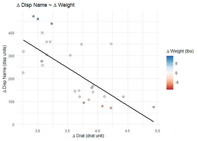
display ggplot without updating values

Hello,

I am investigating linear models of a many different variables, so my ultimate goal is to make many scatterplots with changing variables, labels, and scales. Here is the workflow to do so (edited to do by reprex):
EDIT AGAIN: See display ggplot without updating values - #6 by Megan_Huber comment below for the correct summary of what's happening here - I was wrong about which variables were affected.

library(tidyverse)
library(cowplot)

# define a function to make plots:
gg_lm_simple <- function(.data = ., .y, .x, .var = NULL, .se = FALSE, ...) {
   ggplot(.data, aes(x = {{.x}}, y = {{.y}})) +
      geom_jitter(aes(fill = {{.var}}), shape = 21, na.rm = TRUE, alpha = 0.7, size = 2, ...) +
      geom_smooth(method = "lm", formula = "y ~ x", se = {{.se}}, color = "black", size = 1) +
      scale_fill_distiller(type = "div", palette = "RdBu", 
                           aesthetics = c("fill", "color"), direction = 1,
                           limits = c(-1,1)*max(abs({{.var}}))) + #to keep center at 0, which is necessary for my data
      theme_minimal() +
      labs(title = bquote(Delta ~ .(outcome_oi_name) ~ "~" ~ Delta ~ .(var_oi_name)),
           y = bquote(Delta ~ .(outcome_oi_name) ~ .(outcome_oi_unit)),
           x = bquote(Delta ~ .(indep_oi_name) ~ .(indep_oi_unit)),
           fill = bquote(Delta ~ .(var_oi_name) ~ .(var_oi_unit)))
}

df <- mtcars %>% 
  mutate(wt = (wt-3.2)*4) %>%  #to approximate data that is both positive and negative
  mutate(qsec = qsec-18) #to approximate data that is both positive and negative, smaller scale than qsec

##############################################
#And then this part I copy and paste about 48 times, updating the variables as needed:

# define which of my variables I want to use
outcome_of_interest <- df$disp
outcome_oi_name <- "Disp Name"
outcome_oi_unit <- "(disp units)"
outcome_oi_vlabel <- "disp"
indep_of_interest <- df$drat
indep_oi_name <- "Drat"
indep_oi_unit <- "(drat unit)"
indep_oi_vlabel <- "drat"
var_of_interest <- df$wt
var_oi_name <- "Weight"
var_oi_unit <- "(lbs)"
var_oi_vlabel <- "wt"

splot_out_in_var <- df %>% 
  gg_lm_simple(outcome_of_interest, indep_of_interest, var_of_interest)
# display the plot at this point in the .Rmd
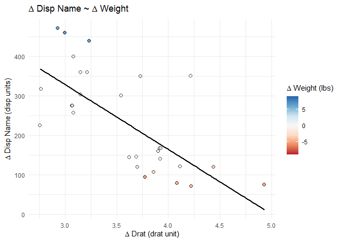
splot_out_in_var 
# save the plot with the specific variable names to use later
assign(glue::glue("splot_{outcome_oi_vlabel}_{indep_oi_vlabel}_{var_oi_vlabel}"), splot_out_in_var)
# so splot_out_in_var would also be assigned to splot_varA_varB_varC
# plus some other code/analysis here, which is not relevent to the question

###############################################
# new variable defined, code is copy/pasted and updated (this will be done about 47 more times)

# define which of my variables I want to use
outcome_of_interest <- df$disp
outcome_oi_name <- "Disp Name"
outcome_oi_unit <- "(disp units)"
outcome_oi_vlabel <- "disp"
indep_of_interest <- df$drat
indep_oi_name <- "Drat"
indep_oi_unit <- "(drat unit)"
indep_oi_vlabel <- "drat"
var_of_interest <- df$qsec
var_oi_name <- "Qsec"
var_oi_unit <- "(units)"
var_oi_vlabel <- "qsec"

splot_out_in_var <- df %>% 
  gg_lm_simple(outcome_of_interest, indep_of_interest, var_of_interest)
# display the plot at this point in the .Rmd
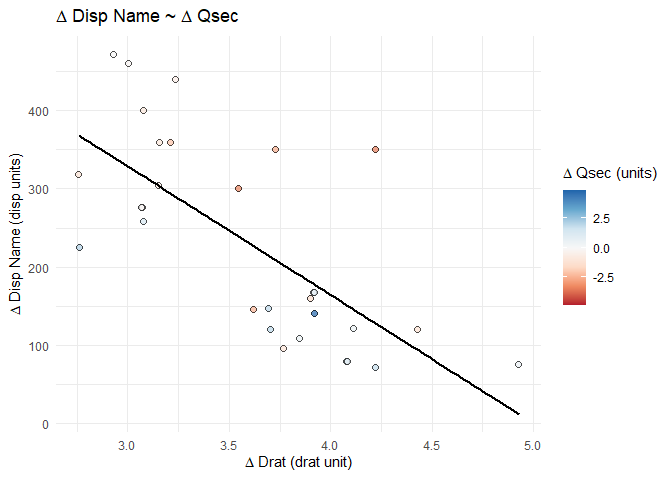
splot_out_in_var 
# save the plot with the specific variable names to use later
assign(glue::glue("splot_{outcome_oi_vlabel}_{indep_oi_vlabel}_{var_oi_vlabel}"), splot_out_in_var)
## so splot_out_in_var would also be assigned to splot_varA_varB_varC
max(abs(var_of_interest))
#> [1] 4.9
max(abs(df$qsec))
#> [1] 4.9

#################################################

#At the end of the Rmd, I want to compare these plots together using cowplot::plot_grid.

# Here I have specifically typed out all 48 names, I'm not using any sort of function to get the names
splot_list <- list(splot_disp_drat_wt, splot_disp_drat_qsec)
# and make the plot:
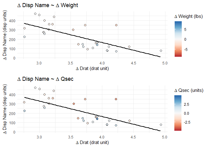
cowplot::plot_grid(plotlist = splot_list, align = "hv", nrow = 2)
Created on 2021-03-11 by the reprex package (v1.0.0)

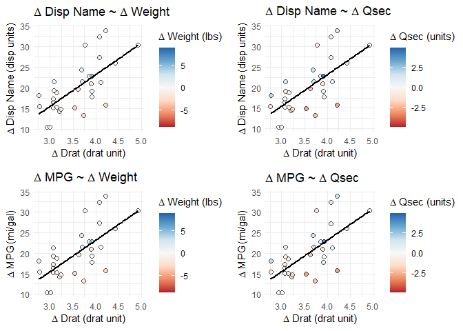
The final plots have the appropriate title and axis names, axis scales, and data points/regression lines. The color/fill scales show the proper values in the legend and the points have the correct relative color for the correct variable, but the actual fill scales are all based on the final plot's variable.

So for a plot that's varA~ varB + varC (where varC goes from -10,10)
When first made, the plot legend will show fill values of c(-10, 10) and the points will be filled such that a point with varC = -10 is darkest red and one with varC = 5 is medium blue, as expected.

However: I then copy/paste, change the outcome/indep/variable_of_interest, and make many new plots (so now the most recent variable_of_interest <- varZ, where varZ goes from -5,5) and call cowplot::plot_grid(). The portion of the plot with varA~ varB + varC has the appropriate titles/labels, the points are filled by varC, the fill legend still shows values from -10 to 10. But the actual scaling of fill values is dictated by varZ, not varC. So a point with varC = -5 is darkest red and one with varC = 5 is darkest blue, but a point where varC = -8 (outside the value range of varZ) is filled grey as if it has a missing varC value. The relationship between the filled points is still relative to varC and not varZ, but the fill scale is set by varZ.

I have no clue how to go from here. Is there a way to assign the ggplot to a variable name and then unlink it somehow, so that calling the variable name will not re-run the gg_lm_simple code but instead just display the saved ggplot object? Or is there something wrong with the way I designed my function so that only the values argument of scale_fill_distiller will be incorrect but everything else is fine?
I guess I could run ggsave() on each plot, then use something to load and grid each image file, but it already takes over 10 minutes to knit and my computer has limited RAM to process loading several hundred images.
See the FAQ: How to do a minimal reproducible example reprex for beginners. You've described the problem well, but having to reverse engineer a script deters interest.

It only needs to contain so much data as will reproduce the undesired result. It doesn't have to be all of your data, or even your data at all. For example, you could use mtcars to do a toy example of the lm modeling chain.

My apologies, I edited the question with reprex!

1 Like

Congratulations, you are the preemptive winner of my 2021 Award for the Best Reprex.

Have you considered making a factory function to spit the plots out with sequentially numbered names plot_1 \dots plot_n in the initial block? Then in any subsequent block, you can call any combination for cowplotting.

As far as the color issue, based on splot_disp_drat_qsec and splot_disp_drat_wt am I right that you're looking for a uniform color scale based on the x-axis that always spans the same range? Think you'd lose anything valuable by discretizing the scale to say 8 increments?

Thanks!
I considered something like the factory function, but this is for a statistics course project (don't worry, I am graded on content, not on code so I'm not cheating!) and I have several plots, linear models, and conceptual questions for each combination of variables so I need to be able to make the plots separately and address the other portions of the assignment before making a new scatterplot. I also need to individually add to the gg_lm_simple plot arguments, like adjusting theme() or adding a geom layer or annotating a certain point.
I'm sure a factory function could work with that, but I am very new to making any sort of function in R and this was already the product of many hours of googling quasiquotation help.

To clarify the color issue: I am comparing scatterplots with the same y and x values, but with fill color set by a third variable var_of_interest, and so I'll ultimately want to have a plot_grid of many scatterplots, with color showing trends for each of these var_of_interests. So if I were using mtcars, I'd have a plot_grid of like y = disp, x = drat, fill = wt or qsec or mpg (etc). So each individual scatterplot needs a scale_fill that maps the values of the var_of_interest, centered around 0.

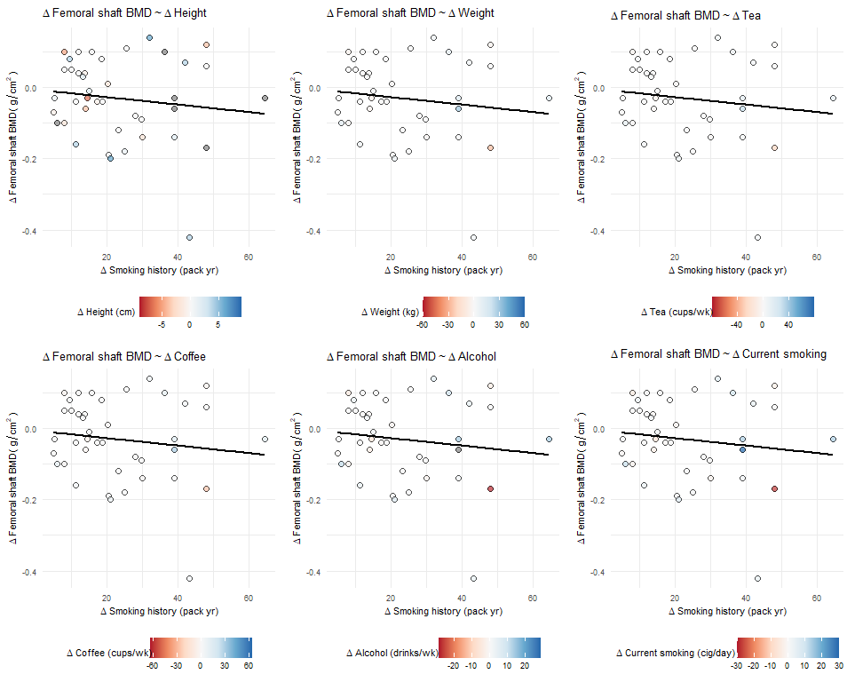
Here is a screenshot of what a current set of these plots looks like. Apologies for the non-reprex, but it's hard to describe it in words. So the fill scale in each of these scatterplots is set by different var_of_intereest and their legends suggest that the colors are scaled appropriately (ex: top left is about (-9, 9), top middle is about (-60, 60)).

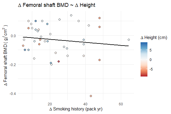
But the actual colors of the points do not match up with the same plots when individually created earlier. For example, the top left plot above, titled "\Delta Femoral shaft BMD ~ \Delta Height", looks like this when first created:
image
The most notable difference is that the plot_grid version has a number of greyed out points, while the original does not.

1 Like

Actually, in taking screenshots to write that previous answer, I think I was incorrect above. It appears that everything besides the fill scale values is based off of the most recent set of outcome_of_interest, indep_of_interest, and var_of_interest. It was hard to see initially because of how I organized the entire Rmarkdown, but (expanding on the above reprex) it's clear that all of these variables are altered to the most recent assignment in the plot_grid() version.

library(tidyverse)
library(cowplot)

# define a function to make plots:
gg_lm_simple <- function(.data = ., .y, .x, .var = NULL, .se = FALSE, ...) {
   ggplot(.data, aes(x = {{.x}}, y = {{.y}})) +
      geom_jitter(aes(fill = {{.var}}), shape = 21, na.rm = TRUE, alpha = 0.7, size = 2, ...) +
      geom_smooth(method = "lm", formula = "y ~ x", se = {{.se}}, color = "black", size = 1) +
      scale_fill_distiller(type = "div", palette = "RdBu", 
                           aesthetics = c("fill", "color"), direction = 1,
                           limits = c(-1,1)*max(abs({{.var}}))) + #to keep center at 0, which is necessary for my data
      theme_minimal() +
      labs(title = bquote(Delta ~ .(outcome_oi_name) ~ "~" ~ Delta ~ .(var_oi_name)),
           y = bquote(Delta ~ .(outcome_oi_name) ~ .(outcome_oi_unit)),
           x = bquote(Delta ~ .(indep_oi_name) ~ .(indep_oi_unit)),
           fill = bquote(Delta ~ .(var_oi_name) ~ .(var_oi_unit)))
}

df <- mtcars %>% 
  mutate(wt = (wt-3.2)*4) %>%  #to approximate data that is both positive and negative
  mutate(qsec = qsec-18) #to approximate data that is both positive and negative, smaller scale than qsec

##############################################
#And then this part I copy and paste, updating the variables as needed:
##FIRST PLOT: disp ~ drat + wt

# define which of my variables I want to use
outcome_of_interest <- df$disp
outcome_oi_name <- "Disp Name"
outcome_oi_unit <- "(disp units)"
outcome_oi_vlabel <- "disp"
indep_of_interest <- df$drat
indep_oi_name <- "Drat"
indep_oi_unit <- "(drat unit)"
indep_oi_vlabel <- "drat"
var_of_interest <- df$wt
var_oi_name <- "Weight"
var_oi_unit <- "(lbs)"
var_oi_vlabel <- "wt"

splot_out_in_var <- df %>% 
  gg_lm_simple(outcome_of_interest, indep_of_interest, var_of_interest)
# display the plot at this point in the .Rmd
splot_out_in_var 

# save the plot with the specific variable names to use later
assign(glue::glue("splot_{outcome_oi_vlabel}_{indep_oi_vlabel}_{var_oi_vlabel}"), splot_out_in_var)
# so splot_out_in_var would also be assigned to splot_disp_drat_wt
# plus some other code/analysis here, which is not relevent to the question

###############################################
# new variable defined, code is copy/pasted and updated
##SECOND PLOT: disp ~ drat + qsec

# define which of my variables I want to use
outcome_of_interest <- df$disp
outcome_oi_name <- "Disp Name"
outcome_oi_unit <- "(disp units)"
outcome_oi_vlabel <- "disp"
indep_of_interest <- df$drat
indep_oi_name <- "Drat"
indep_oi_unit <- "(drat unit)"
indep_oi_vlabel <- "drat"
var_of_interest <- df$qsec
var_oi_name <- "Qsec"
var_oi_unit <- "(units)"
var_oi_vlabel <- "qsec"

splot_out_in_var <- df %>% 
  gg_lm_simple(outcome_of_interest, indep_of_interest, var_of_interest)
# display the plot at this point in the .Rmd
splot_out_in_var 

# save the plot with the specific variable names to use later
assign(glue::glue("splot_{outcome_oi_vlabel}_{indep_oi_vlabel}_{var_oi_vlabel}"), splot_out_in_var)
## so splot_out_in_var would also be assigned to splot_disp_drat_qsec

##############################################
#And then this part I copy and paste, updating the variables as needed:
##THIRD PLOT: mpg ~ drat + wt

# define which of my variables I want to use
outcome_of_interest <- df$mpg
outcome_oi_name <- "MPG"
outcome_oi_unit <- "(mi/gal)"
outcome_oi_vlabel <- "mpg"
indep_of_interest <- df$drat
indep_oi_name <- "Drat"
indep_oi_unit <- "(drat unit)"
indep_oi_vlabel <- "drat"
var_of_interest <- df$wt
var_oi_name <- "Weight"
var_oi_unit <- "(lbs)"
var_oi_vlabel <- "wt"

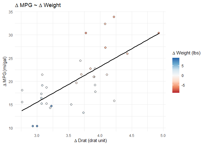
splot_out_in_var <- df %>% 
  gg_lm_simple(outcome_of_interest, indep_of_interest, var_of_interest)
# display the plot at this point in the .Rmd
splot_out_in_var 

# save the plot with the specific variable names to use later
assign(glue::glue("splot_{outcome_oi_vlabel}_{indep_oi_vlabel}_{var_oi_vlabel}"), splot_out_in_var)
# so splot_out_in_var would also be assigned to splot_mpg_drat_wt
# plus some other code/analysis here, which is not relevent to the question

###############################################
# new variable defined, code is copy/pasted and updated
##FOURTH PLOT: mpg ~ drat + qsec

outcome_of_interest <- df$mpg
outcome_oi_name <- "MPG"
outcome_oi_unit <- "(mi/gal)"
outcome_oi_vlabel <- "mpg"
indep_of_interest <- df$drat
indep_oi_name <- "Drat"
indep_oi_unit <- "(drat unit)"
indep_oi_vlabel <- "drat"
var_of_interest <- df$qsec
var_oi_name <- "Qsec"
var_oi_unit <- "(units)"
var_oi_vlabel <- "qsec"

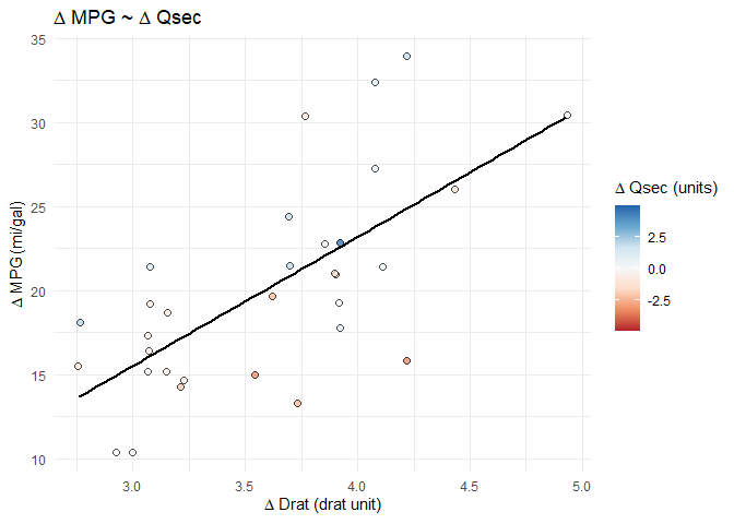
splot_out_in_var <- df %>% 
  gg_lm_simple(outcome_of_interest, indep_of_interest, var_of_interest)
# display the plot at this point in the .Rmd
splot_out_in_var 

# save the plot with the specific variable names to use later
assign(glue::glue("splot_{outcome_oi_vlabel}_{indep_oi_vlabel}_{var_oi_vlabel}"), splot_out_in_var)
## so splot_out_in_var would also be assigned to splot_disp_drat_qsec

#################################################

#At the end of the Rmd, I want to compare these plots together using cowplot::plot_grid.

# Here I have specifically typed out all 48 names, I'm not using any sort of function to get the names
splot_list <- list(splot_disp_drat_wt, splot_disp_drat_qsec,
                   splot_mpg_drat_wt, splot_mpg_drat_qsec)
# and make the plot:
cowplot::plot_grid(plotlist = splot_list, align = "hv", nrow = 2)

Created on 2021-03-11 by the reprex package (v1.0.0)
So even though the graph labels remain as they should, all four plots are clearly plotting mpg as the y axis since the top two graphs should have negative slopes.

1 Like

So my initial question stands: how do I save each individual ggplot object as a variable instead of the ggplot code? Or is there a different way to avoid re-plotting the plots when I place them in cowplot::plot_grid()?

This topic was automatically closed 21 days after the last reply. New replies are no longer allowed.

If you have a query related to it or one of the replies, start a new topic and refer back with a link.