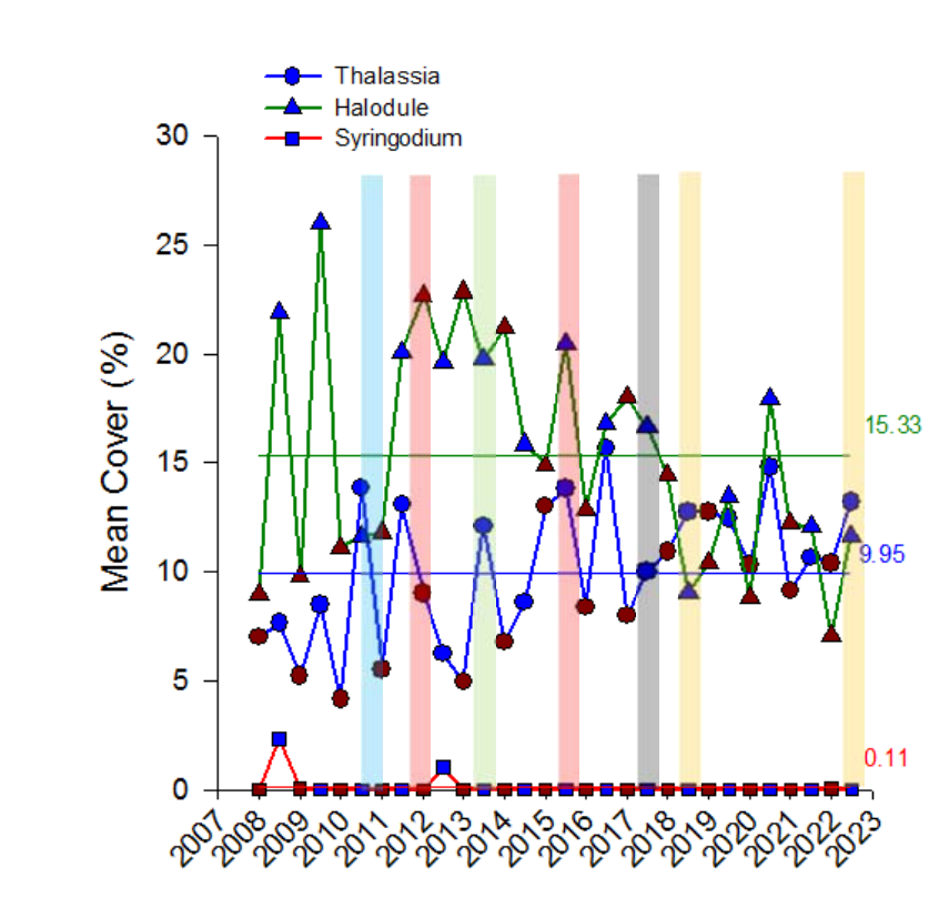
I'm trying to give my geom_line and geom_point different colors based on 2 different columns, but can't over-ride the aesthetics of the first. If I hope to re-create this plot (below), how would I assign the colors of the line to be by the factor levels of "SAV" and the colors of the points to be by "Season"? The "Season" colors shouldn't show up in the legend though. Thank you!
library(ggplot2)

ggplot(cdata2, aes(x = CYR, y = n_mean)) +
    annotate(geom = "rect", xmin = 2010, xmax = 2010.25, ymin = -Inf, ymax = Inf,
             fill = "lightblue", colour = NA, alpha = 0.4) +
    annotate(geom = "rect", xmin = 2013.5, xmax = 2013.75, ymin = -Inf, ymax = Inf,
             fill = "lightgreen", colour = NA, alpha = 0.4) +
    annotate(geom = "rect", xmin = 2017.5, xmax = 2017.75, ymin = -Inf, ymax = Inf,
             fill = "#E0E0E0", colour = NA, alpha = 0.4) +
    annotate(geom = "rect", xmin = 2011.5, xmax = 2011.75, ymin = -Inf, ymax = Inf,
             fill = "pink", colour = NA, alpha = 0.4) +
    annotate(geom = "rect", xmin = 2015.5, xmax = 2015.75, ymin = -Inf, ymax = Inf,
             fill = "pink", colour = NA, alpha = 0.4) +
    annotate(geom = "rect", xmin = 2018.5, xmax = 2018.75, ymin = -Inf, ymax = Inf,
             fill = "orange", colour = NA, alpha = 0.2) +
    annotate(geom = "rect", xmin = 2022.5, xmax = 2022.75, ymin = -Inf, ymax = Inf,
           fill = "orange", colour = NA, alpha = 0.2) +


    # Color lines by SAV values (put in legend)
    geom_line(aes(y = n_mean, color = SAV), size = 1) +

    # Grand mean (straight line); color lines by SAV levels (Not in legend)
    geom_line(data = cdata2, aes(y=grand_mean, color = SAV), linewidth = 0.75) +

    # Color points by season (not in legend). Blue and red.
    geom_point(aes(y=n_mean, shape=SAV, color = Season), size = 3) +


    # To avoid having 2 legends, color_manual and shape_manual need to be the same?
    scale_color_manual(labels=c('Thalassia', 'Halodule', 'Syringodium'),
                       values=c("red", "dark green", "blue", "dark blue", "dark red"),
                       breaks=c("ave_tt", "ave_hw", "ave_sf")) +

    scale_shape_manual(labels=c('Thalassia', 'Halodule', 'Syringodium'),
                       values = c(17,15,16), # Triangle, circle, square
                       breaks=c("ave_tt", "ave_hw", "ave_sf")) +

    scale_x_continuous(
                       breaks = c(2007,2008,2009,2010,2011,2012,2013,2014,2015,2016,
                                  2017,2018,2019,2020,2021,2022,2023),
                       # Tick marks

                       limits = c(2007,2023),
                       # Start and end from 2007 to 2023 (better than xlim())

                       labels = c(2007,2008,2009,2010,2011,2012,2013,2014,2015,2016,
                                  2017,2018,2019,2020,2021,2022,2023),
                       expand=c(0, 0)) +
                       # Start origin @ first break,
                       # c(-1,0) starts 2022 at origin and goes backwards!
                       # c(1<-0,0) squishes the plot long-way inward

  scale_y_continuous(
    expand = c(0, 0), # x-axis starts @ y=0
    limits = c(0, 30), # 0->1 y-axis
    breaks = c(0,5,10,15,20,25,30)) +  # y-axis step

    theme(panel.border = element_rect(fill = NA, color = "black"),
          panel.background = element_blank(),
          panel.grid.major = element_blank(),
          panel.grid.minor = element_blank(),
          plot.title = element_text(hjust = 0.5),
          axis.text.y = element_text(size = 11, face = "bold"),
          axis.text.x = element_text(size = 10, vjust = 1.0, hjust=1.0, angle = 45, face = "bold"), # hjust: Close to 1.0 = Left
          axis.title = element_text(size = 14, face = "bold"),
          legend.title=element_blank()) +
    labs(x= NULL, y = "SAV (ave. % cover)") +

    # Geom text for grand means
    geom_text(data = cdata3, aes(label = paste0(round(n_mean[1],2)), x = 2022, y=17), color = "dark green")+
    geom_text(data = cdata3, aes(label = paste0(round(n_mean[3],2)), x = 2022, y=14.5), color = "blue")+
    geom_text(data = cdata3, aes(label = paste0(round(n_mean[2],2)), x = 2022, y=2), color = "red")
Data (2 dataframes):
> dput(cdata3)
structure(list(SAV = c("ave_hw", "ave_sf", "ave_tt"), N = c(286935L,
286935L, 286935L), n_mean = c(15.3737370343434, 0.114431692544803,
9.95752343992832)), class = "data.frame", row.names = c(NA, -3L
))

> dput(cdata2)
structure(list(CYR = c(2007, 2007, 2007, 2007.5, 2007.5, 2007.5,
2008, 2008, 2008, 2008.5, 2008.5, 2008.5, 2009, 2009, 2009, 2009.5,
2009.5, 2009.5, 2010, 2010, 2010, 2010.5, 2010.5, 2010.5, 2011,
2011, 2011, 2011.5, 2011.5, 2011.5, 2012, 2012, 2012, 2012.5,
2012.5, 2012.5, 2013, 2013, 2013, 2013.5, 2013.5, 2013.5, 2014,
2014, 2014, 2014.5, 2014.5, 2014.5, 2015, 2015, 2015, 2015.5,
2015.5, 2015.5, 2016, 2016, 2016, 2016.5, 2016.5, 2016.5, 2017,
2017, 2017, 2017.5, 2017.5, 2017.5, 2018, 2018, 2018, 2018.5,
2018.5, 2018.5, 2019, 2019, 2019, 2019.5, 2019.5, 2019.5, 2020,
2020, 2020, 2020.5, 2020.5, 2020.5, 2021, 2021, 2021, 2021.5,
2021.5, 2021.5, 2022, 2022, 2022, 2022.5, 2022.5, 2022.5), Season = c("DRY",
"DRY", "DRY", "WET", "WET", "WET", "DRY", "DRY", "DRY", "WET",
"WET", "WET", "DRY", "DRY", "DRY", "WET", "WET", "WET", "DRY",
"DRY", "DRY", "WET", "WET", "WET", "DRY", "DRY", "DRY", "WET",
"WET", "WET", "DRY", "DRY", "DRY", "WET", "WET", "WET", "DRY",
"DRY", "DRY", "WET", "WET", "WET", "DRY", "DRY", "DRY", "WET",
"WET", "WET", "DRY", "DRY", "DRY", "WET", "WET", "WET", "DRY",
"DRY", "DRY", "WET", "WET", "WET", "DRY", "DRY", "DRY", "WET",
"WET", "WET", "DRY", "DRY", "DRY", "WET", "WET", "WET", "DRY",
"DRY", "DRY", "WET", "WET", "WET", "DRY", "DRY", "DRY", "WET",
"WET", "WET", "DRY", "DRY", "DRY", "WET", "WET", "WET", "DRY",
"DRY", "DRY", "WET", "WET", "WET"), SAV = c("ave_hw", "ave_sf",
"ave_tt", "ave_hw", "ave_sf", "ave_tt", "ave_hw", "ave_sf", "ave_tt",
"ave_hw", "ave_sf", "ave_tt", "ave_hw", "ave_sf", "ave_tt", "ave_hw",
"ave_sf", "ave_tt", "ave_hw", "ave_sf", "ave_tt", "ave_hw", "ave_sf",
"ave_tt", "ave_hw", "ave_sf", "ave_tt", "ave_hw", "ave_sf", "ave_tt",
"ave_hw", "ave_sf", "ave_tt", "ave_hw", "ave_sf", "ave_tt", "ave_hw",
"ave_sf", "ave_tt", "ave_hw", "ave_sf", "ave_tt", "ave_hw", "ave_sf",
"ave_tt", "ave_hw", "ave_sf", "ave_tt", "ave_hw", "ave_sf", "ave_tt",
"ave_hw", "ave_sf", "ave_tt", "ave_hw", "ave_sf", "ave_tt", "ave_hw",
"ave_sf", "ave_tt", "ave_hw", "ave_sf", "ave_tt", "ave_hw", "ave_sf",
"ave_tt", "ave_hw", "ave_sf", "ave_tt", "ave_hw", "ave_sf", "ave_tt",
"ave_hw", "ave_sf", "ave_tt", "ave_hw", "ave_sf", "ave_tt", "ave_hw",
"ave_sf", "ave_tt", "ave_hw", "ave_sf", "ave_tt", "ave_hw", "ave_sf",
"ave_tt", "ave_hw", "ave_sf", "ave_tt", "ave_hw", "ave_sf", "ave_tt",
"ave_hw", "ave_sf", "ave_tt"), N = c(8695L, 8695L, 8695L, 8695L,
8695L, 8695L, 8695L, 8695L, 8695L, 8695L, 8695L, 8695L, 8695L,
8695L, 8695L, 8695L, 8695L, 8695L, 8695L, 8695L, 8695L, 8695L,
8695L, 8695L, 8695L, 8695L, 8695L, 8695L, 8695L, 8695L, 8695L,
8695L, 8695L, 8695L, 8695L, 8695L, 8695L, 8695L, 8695L, 8695L,
8695L, 8695L, 8695L, 8695L, 8695L, 8695L, 8695L, 8695L, 8695L,
8695L, 8695L, 8695L, 8695L, 8695L, 8695L, 8695L, 8695L, 8695L,
8695L, 8695L, 8695L, 8695L, 8695L, 8695L, 8695L, 8695L, 8695L,
8695L, 8695L, 8695L, 8695L, 8695L, 8695L, 8695L, 8695L, 8695L,
8695L, 8695L, 8695L, 8695L, 8695L, 8695L, 8695L, 8695L, 8695L,
8695L, 8695L, 17390L, 17390L, 17390L, 8695L, 8695L, 8695L, 8695L,
8695L, 8695L), n_mean = c(NaN, NaN, NaN, NaN, NaN, NaN, 8.98527191489362,
0, 6.98, 21.8943971553191, 2.3153427893617, 7.64548463829787,
9.77706959380851, 0.0319148936170213, 5.21412959574468, 26.0077821638298,
0, 8.45628615744681, 11.1126796764706, 0.00588235294117647, 4.133759,
11.6129787234043, 0, 13.866170212766, 11.8146809347826, 0, 5.52577639782609,
20.0829787234043, 0, 13.0765957446809, 22.6851063829787, 0, 9.02340425531915,
19.6428446808511, 1.03215106382979, 6.23103829787234, 23.0308695652174,
0, 3.02434782608696, 19.7425531914894, 0, 12.098085106383, 21.1297872340426,
0, 6.91914893617021, 15.8510638297872, 0, 8.59148936170213, 14.9243498297872,
0, 13.0065012765957, 20.4765957446808, 0, 13.8042553191489, 12.8574468085106,
0, 8.36808510638298, 16.768085106383, 0, 15.6893617021277, 18.0154255319149,
0, 7.97234042553191, 16.6425531914894, 0, 9.99574468085106, 14.4212765957447,
0, 10.9170212765957, 9.05957446808511, 0, 12.7340425531915, 10.3893617021277,
0, 12.7276595744681, 13.4364065957447, 0, 12.4276595744681, 8.78936170212766,
0.00212765957446809, 10.3127659574468, 17.968085106383, 0, 14.7765957446809,
12.2234042553191, 0, 9.12765957446809, 12.0808510638298, 0, 10.6574468085106,
7.06808510638298, 0.0106382978723404, 10.3914893617021, 11.6297872340426,
0, 13.1787234042553), n_median = c(NA, NA, NA, NA, NA, NA, 3,
0, 2.32, 20.7, 0, 0.2, 6.6, 0, 1.51, 26, 0, 2.71, 10.4, 0, 1.4772725,
6.6, 0, 5.5, 7.9785715, 0, 0.55, 18, 0, 1.1, 13.5, 0, 2.1, 19.5,
0, 1.8, 22.75, 0, 0.05, 19.1, 0, 0.6, 19, 0, 1.5, 10.7, 0, 1,
12, 0, 8, 13, 0, 7.5, 11, 0, 3.5, 16.2, 0, 8.6, 16.5, 0, 0.6,
14.1, 0, 0.5, 12, 0, 6.5, 8, 0, 5, 8.2, 0, 4.3, 11.6, 0, 8.8,
6.8, 0, 6.5, 19, 0, 11.5, 10.1, 0, 5.7, 8.7, 0, 4.7, 5, 0, 4.1,
9.5, 0, 3), sd = c(NA, NA, NA, NA, NA, NA, 11.7085445738399,
0, 11.7037840986077, 20.9798396749426, 10.4019772483536, 10.7510377253969,
9.45639825464561, 0.21646978819132, 8.50015402914711, 23.4389588168003,
0, 11.951876499548, 9.07443174861995, 0.0235312823702472, 5.14547979546789,
12.4331709472457, 0, 15.7887893178601, 13.3600974353576, 0, 8.86461330488266,
18.2140229059275, 0, 18.0923244678731, 24.2988009061075, 0, 12.5755580996472,
15.6950429641397, 6.36880461080622, 7.76768756867771, 14.8923349009443,
0, 5.78304099792998, 14.3358394751566, 0, 16.6545356701125, 16.5113577583701,
0, 10.4140034508656, 16.0767802318981, 0, 12.6812861503859, 14.8715784407585,
0, 14.8710278913095, 20.0770341464803, 0, 15.5527562398657, 11.3350420672201,
0, 11.3192875331138, 15.1709732834689, 0, 18.2528957714625, 16.4433980698121,
0, 12.017818981421, 15.7909769267971, 0, 15.8837685790693, 14.142045197017,
0, 15.6274080485381, 8.84612691530042, 0, 17.0140681969259, 10.1987764434213,
0, 15.6842268952042, 11.6353578097032, 0, 14.0963614866631, 7.50745634994085,
0.0144313192127546, 12.1654309051214, 13.4313362297506, 0, 16.249629491747,
10.4357129517743, 0, 10.7546123117319, 10.6263854112514, 0, 13.699083133139,
7.87975827536278, 0.0721565960637732, 13.3007061558202, 10.4435339370082,
0, 19.2295746932576), se = c(NA, NA, NA, NA, NA, NA, 0.125564861065502,
0, 0.125513808741503, 0.224992153153388, 0.111552962006418, 0.115296358978348,
0.101412376707997, 0.00232146691740417, 0.0911574152512433, 0.251364256999733,
0, 0.128174403118456, 0.097316088654574, 0.000252354353940351,
0.0551811928082687, 0.133335904624953, 0, 0.169322252188291,
0.143276456583713, 0, 0.0950659521349834, 0.19533096032589, 0,
0.194025841028627, 0.260585381948376, 0, 0.134862893986958, 0.168316896842368,
0.0683003819190261, 0.083302292971616, 0.159708489042777, 0,
0.0620185314119729, 0.153740516646043, 0, 0.178606695677658,
0.17707122604843, 0, 0.111681933497115, 0.172410726497054, 0,
0.13599674353743, 0.159485892457608, 0, 0.159479988251101, 0.215310279370048,
0, 0.166790984492437, 0.121559342697649, 0, 0.121390387805456,
0.162696664863314, 0, 0.195747841000456, 0.176342412249412, 0,
0.128881583974495, 0.169345712560374, 0, 0.170340829489904, 0.151662226602697,
0, 0.16759156597591, 0.0948677002579155, 0, 0.182462397083852,
0.109373794418269, 0, 0.1682009030752, 0.124779991023567, 0,
0.151172305015315, 0.0805115193942914, 0.000154764461160278,
0.130464604867841, 0.144040436193989, 0, 0.174264397818995, 0.111914750688714,
0, 0.115334693583787, 0.0805815788598744, 0, 0.103882336756974,
0.084504162480305, 0.000773822305801391, 0.142639532180634, 0.111998624556905,
0, 0.206221948379678), grand_mean = c(NA, NA, NA, NA, NA, NA,
15.3737370343434, 0.114431692544803, 9.95752343992832, 15.3737370343434,
0.114431692544803, 9.95752343992832, 15.3737370343434, 0.114431692544803,
9.95752343992832, 15.3737370343434, 0.114431692544803, 9.95752343992832,
15.3737370343434, 0.114431692544803, 9.95752343992832, 15.3737370343434,
0.114431692544803, 9.95752343992832, 15.3737370343434, 0.114431692544803,
9.95752343992832, 15.3737370343434, 0.114431692544803, 9.95752343992832,
15.3737370343434, 0.114431692544803, 9.95752343992832, 15.3737370343434,
0.114431692544803, 9.95752343992832, 15.3737370343434, 0.114431692544803,
9.95752343992832, 15.3737370343434, 0.114431692544803, 9.95752343992832,
15.3737370343434, 0.114431692544803, 9.95752343992832, 15.3737370343434,
0.114431692544803, 9.95752343992832, 15.3737370343434, 0.114431692544803,
9.95752343992832, 15.3737370343434, 0.114431692544803, 9.95752343992832,
15.3737370343434, 0.114431692544803, 9.95752343992832, 15.3737370343434,
0.114431692544803, 9.95752343992832, 15.3737370343434, 0.114431692544803,
9.95752343992832, 15.3737370343434, 0.114431692544803, 9.95752343992832,
15.3737370343434, 0.114431692544803, 9.95752343992832, 15.3737370343434,
0.114431692544803, 9.95752343992832, 15.3737370343434, 0.114431692544803,
9.95752343992832, 15.3737370343434, 0.114431692544803, 9.95752343992832,
15.3737370343434, 0.114431692544803, 9.95752343992832, 15.3737370343434,
0.114431692544803, 9.95752343992832, 15.3737370343434, 0.114431692544803,
9.95752343992832, 15.3737370343434, 0.114431692544803, 9.95752343992832,
15.3737370343434, 0.114431692544803, 9.95752343992832, 15.3737370343434,
0.114431692544803, 9.95752343992832)), row.names = c(NA, -96L
), class = "data.frame")