Determining the Overall Slope of a GAM Model

brant · December 19, 2023, 5:52pm

I am sorry that I have posted this issue in two places, I know that this isn't proper practice, but it is not allowing me to edit my previous post.

I am trying to determine the slope of two GAM models and compare how the slope changes between models.

I created GAM models looking at the relationship between precipitation and stream discharge under a pre-and post-treatment scenario. The pre-treatment model is named "preGAM" and the post-treatment model is named "postGAM". The code used to create these models is provided below.

I first created both GAM models using the following code:

preGAM <- gam(preGAM.dat$DailyIncrease ~ s(preGAM.dat$Precipitation, method = "REML"))

postGAM <- gam(postGAM.dat$DailyIncrease ~ s(postGAM.dat$Precipitation, method = "REML"))

I then viewed the summary of the model "preGAM", which returned the following output:

> summary(preGAM) 

Family: gaussian 
Link function: identity 

Formula:
preOutlierRem.dat$DailyIncrease ~ s(preOutlierRem.dat$Precipitation)

Parametric coefficients:
              Estimate  Std. Error t value Pr(>|t|)    
(Intercept)   0.1275     0.0186   6.853 1.97e-11 ***
---
Signif. codes:  0 ‘***’ 0.001 ‘**’ 0.01 ‘*’ 0.05 ‘.’ 0.1 ‘ ’ 1

Approximate significance of smooth terms:
                                     edf Ref.df    F p-value    
s(preOutlierRem.dat$Precipitation) 6.102  7.195 40.2  <2e-16 ***
---
Signif. codes:  0 ‘***’ 0.001 ‘**’ 0.01 ‘*’ 0.05 ‘.’ 0.1 ‘ ’ 1

R-sq.(adj) =  0.347   Deviance explained = 35.4%
-REML = 335.04  Scale est. = 0.18963   n = 548```

I then viewed the summary for the model "postGAM", which returned the following output:

Family: gaussian 
Link function: identity 

Formula:
postOutlierRem.dat$DailyIncrease ~ s(postOutlierRem.dat$Precipitation)

Parametric coefficients:
             Estimate Std. Error t value Pr(>|t|)    
(Intercept)  0.13046    0.01273   10.25   <2e-16 ***
---
Signif. codes:  0 ‘***’ 0.001 ‘**’ 0.01 ‘*’ 0.05 ‘.’ 0.1 ‘ ’ 1

Approximate significance of smooth terms:
                                      edf Ref.df     F p-value    
s(postOutlierRem.dat$Precipitation) 8.836  8.991 101.2  <2e-16 ***
---
Signif. codes:  0 ‘***’ 0.001 ‘**’ 0.01 ‘*’ 0.05 ‘.’ 0.1 ‘ ’ 1

R-sq.(adj) =  0.452   Deviance explained = 45.6%
-REML = 636.78  Scale est. = 0.17773   n = 1097

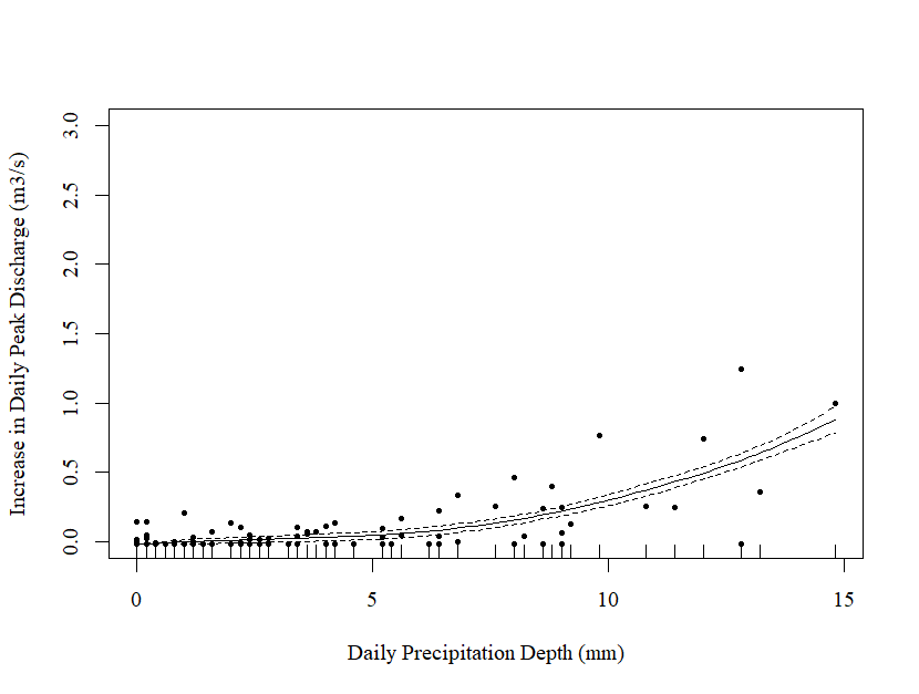
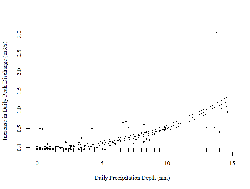
I then plotted each relationship as shown in Figures 1 and 2 below:

Figure 1: Relationship Between Daily Precipitation Depth (mm) and the Increase in Daily Peak Discharge (m3/s) Pre-Treatment

Figure 2: Relationship Between Daily Precipitation Depth (mm) and the Increase in Daily Peak Discharge (m3/s) Post-Treatment

I am now trying to make sense of these outputs and determine how to 1) understand the preGAM relationship between the variables Precipitation and Daily Increase, 2) understand the postGAM relationship between the variables Precipitation and Daily Increase, and 3) make observations as to if and how the relationship between Precipitation and Daily Increase preGAM and postGAM differ.

I began by looking at the significance of the significance of the smoothed term for precipitation in both models. As shown in the output above, the smoothed term for precipitation was highly significant for both the preGAM (p < 2e-16) and postGAM (p <2e-16) scenarios.

As I understand it, the value of the effective degrees of freedom (edf) represents the order of the relationship, where an EDF of 1 is equivalent to a linear relationship, an edf of 2 is equivalent to a quadratic curve, and so on, with higher edfs describing more "wiggly" curves.

Therefore, my preGAM model has been fitted an order 6 (edf = 6.102) relationship, and my postGAM model has been fitted to an order 9 (edf = 8.836) relationship. As the p-value for the approximate significance of the smoothed term (precipitation) for the preGAM model is <2e-16, and and the p-value for the approximate significance for the smoothed term (precipitation) for the postGAM model is <2e-16. I know that for both models, the relationship between daily precipitation depth and the increase in daily stream discharge is highly significant (which makes sense logically). I believe that for comparison these should have the same model order in order to accurately compare the slopes.

My remaining questions are:

Does anyone have any advice on how to revise the models to ensure that both models (pre-GAM and post-GAM) are of the same order?
Does anyone have any advice on how to determine the overall slope of the models

I want to create two models of the same model order, and compare the slopes of these models to determine if the relationship between daily precipitation depth and daily peak stream discharge is different in the post development scenario (compared to the pre-development scenario). I appreciate any advice that anyone might have.

TIA

mcneills · December 20, 2023, 3:01am

I would have thought the easiest way to proceed is to combine pre- and post-treatment data into a single data frame, with the distinction between the two determined by some factor (let's say, for the sake of argument, "treated" with values "Pre" and "Post"). I guess this could be generated with something like this:

df <- bind_rows(bind_cols(treatment="Pre",preGAM.dat),bind_cols(treatment="Post",postGAM.dat))

Then, it would be possible to consider the effect of the pre/post treatment. How that is done depends on how you expect the treatment to affect the precipitation). Something like the following is my (naiive) view of how it could be done:

mgam <- gam(DailyIncrease ~ s(Precipitation) + treatment,data=df,method="REML")

...which would suggest an additive effect for the treatment. I have no idea whether this is likely or not... But you could also have the GAM vary by treatment:

df$treatment <- factor(df$treatment,levels=c("Pre","Post")
mgam2 <- gam(DailyIncrease ~ s(Precipitation,by=treatment),data=df,method="REML")

Only you can say which of these models makes more sense, and how to interpret the treatment in each.

Note that I think it is unlikely that you would treat the response variable as Gaussian - the data looks right skewed to me. One suggestion would be to use a Gamma with a log-link. Using the last model as an example, you would use:

mgam3 <- gam(DailyIncrease ~ s(Precipitation,by=treatment),data=df,method="REML",family=Gamma(link=log)

...which makes more sense to me.

Also, since the data is fairly noisy with respect to precipitation, you might want to constrain the knots in the smooth function. But, a bit of experimentation is required.

Good luck
Stephen

brant · December 21, 2023, 7:47pm

Thank you,

I have combined the pre- and post- treatment data into a single data frame as you suggested. I think that I would want the GAM to vary by treatment as I am trying to compare how the effect of Precipitation on DailyIncrease, changes before (i.e., "Pre") compared to after (i.e., "Post") treatment.

As such, I used the following code to create my GAM models.

First I combined the "Pre" and "Post" data into a single data frame using the code:

df <- bind_rows(bind_cols(treatment="Pre", preOutlierRem.dat), bind_cols(treatment="Post", postOutlierRem.dat))

I then used the following code to create a data frame with levels "Pre" and "Post" using the code:

df$treatment <- factor(df$treatment,levels=c("Pre", "Post")

This has properly combined my pre- and post-treatment data into a single data frame with the format:

treatment  Date           Discharge    Precipitation   DailyChange   DailyIncrease
Pre        2010-05-01     0.941        2.8                   0.000        0.000
Pre        2010-05-02     0.528        28.8                 -0.413        0.000
Pre        2010-05-03     0.422        0.0                  -0.106        0.000
Pre        2010-05-04     0.366        2.8                  -0.056        0.000
Pre        2010-05-05     1.381        12.0                  1.015        1.015

I then tried to create a GAM model where the Daily Increase in stream discharge was a function of precipitation depth, and had the GAM vary by treatement (i.e., I expect the relationship between precipitation depth and the daily increase in stream discharge to be vary depending on if it was pre- or post treatment)

To do so, I used the code

mgam2 <- gam(DailyIncrease ~ s(Precipitation,by=treatment), data=df, method="REML") family=Gamma(link=log))```

When I run the above line of code, I receive the error "Error in eval(family$initialize) : non-positive values not allowed for the 'Gamma' family"

I believe that this is because the "DailyChange" column in my data frame has positive and negative values. Is there a way to remove the column "DailyChange" from my data frame so that I only have the columns "treatment", "Date", "Discharge", "Precipitation", and "Daily Increase"?

mcneills · December 21, 2023, 11:03pm

I don't think the problem is that DailyChange has negative values, because that variable is not inclued in your GAM. However, it does suggest that you have negative or zero values in DailyIncrease in this data frame.

If the negative values are a mistake, they could be removed. If they really are important, you'll have to find another distribution for the response. If you're still concerned about the non-constant variance, you might have to apply some kind of transformation that can handle positive and negative values. Such transformations do exist, but you'd need to think about the problem a bit more.

brant · December 22, 2023, 11:07pm

Thank you. I do not have any negative values in the "DailyIncrease" variable, but I do have several values of zero. Would zero values cause the error "Error in eval(family$initialize) : non-positive values not allowed for the 'Gamma' family"?

benjaminhlina · January 2, 2024, 3:26pm

The 0 values will create an error considering the link function is set to log. You may be able to use identity as link function for the Gamma() family but that may not be appropriate for the distribution of the data. You may want to look into the package {brms} which can fit a Gamma-Hurdle model that takes account of the 0 in your data and can fit smoothers.

One suggestion to the above code that @mcneills provided is that if you are to add in treatment you will more than likely want to set the y-intercepts to be separate. You can do this by having treatment as a covariate and as the by argument. See below example using your variables:

m <- gam(DailyIncrease ~ treatment + s(Precipitation, by = treatment), 
         data = df, 
         method = "REML", 
         family = Gamma(link = log))

Good luck and happy GAMing!

brant · January 8, 2024, 4:26pm

Thank you. That worked, I am still unsure as to how to determine the overall slopes of both the preGAM15 and postGAM15 models and determine if these slopes are significantly different. Does anyone have any advice?

I had very few precipitation events greater than 15 mm in precipitation depth, so I removed all observations with precipitation events greater than 15 mm and created four data objects looking at precipitation depth and the increase in stream discharge for events less than 15 mm. This was achieved using the code below, where prePrecip15 is daily precipitation depth of events less than 15 mm between 2010 and 2012, preIncrease15 is the increase in stream discharge for each precipitation event less than 15 mm between 2010 and 2012, postPrecip15 is the daily precipitation depth of events less than 15 mm between 2020 and 2022, and postIncrease15 the daily increase in stream discharge for each precipitation event less than 15 mm between 2010 and 2022 (see code below).

prePrecip15 <- preOutlierRem.dat$Precipitation[which(preOutlierRem.dat$Precipitation < 15)]
preIncrease15 <- preOutlierRem.dat$DailyIncrease[which(preOutlierRem.dat$Precipitation < 15)]

postPrecip15 <- postOutlierRem.dat$Precipitation[which(postOutlierRem.dat$Precipitation < 15)]
postIncrease15 <- postOutlierRem.dat$DailyIncrease[which(postOutlierRem.dat$Precipitation < 15)]

I then used this data to create two GAM models (one for the relationship between precipitation depth and the daily increase in stream discharge between 2010 and 2012 (i.e., preGAM) and the other for the relationship between precipitation depth and the daily increase in stream discharge between 2020 and 2022 (i.e., postGAM) using the code below:

preGAM15 <- gam(preIncrease15 ~ s(prePrecip15), method = "REML")
postGAM15 <- gam(postIncrease15 ~ s(postPrecip15), method = "REML")

I then looked at the summary of each model and found that the preGAM15 model had an r-squared value of 0.623 and the postGAM15 model had an r-squared value of 0.617 (which isn't great but is acceptable).

I then plotted the residuals around the preGAM15 and postGAM15 models to observe the trend of the model and model residuals using the code:

plot.gam(preGAM15, residuals = TRUE, xlab = "Daily Precipitation Depth (mm)", ylab = "Increase in Daily Peak Discharge (m3/s)", family = "A", pch = 19, cex = .5, ylim = c(0,3))
plot.gam(postGAM15, residuals = TRUE, xlab = "Daily Precipitation Depth (mm)", ylab = "Increase in Daily Peak Discharge (m3/s)", family = "A", pch = 19, cex = .5, ylim = c(0,3))

This returned the following plots

Figure 1: preGAM15 model comparing the relationship between daily precipitation depth and the daily increase in stream discharge between 2010 and 2012.

Figure 2: postGAM15 model comparing the relationship between daily precipitation depth and the daily increase in stream discharge between 2020 and 2022.

I then viewed the slope coefficients of the preGAM15 and postGAM15 models using the code:

preGAM15$coefficients
postGAM15$coefficients

This returned the following output for the preGAM15 model

     (Intercept) s(prePrecip15).1 s(prePrecip15).2 s(prePrecip15).3 s(prePrecip15).4 
      0.01890256       0.08645833      -0.24569476       0.13332839       0.19350182 
s(prePrecip15).5 s(prePrecip15).6 s(prePrecip15).7 s(prePrecip15).8 s(prePrecip15).9 
      0.13919646      -0.18811312      -0.15779142      -0.83407930       0.18684002

and the following output for the postGAM15 model:

      (Intercept) s(postPrecip15).1 s(postPrecip15).2 s(postPrecip15).3 s(postPrecip15).4 
       0.03787266        0.10965270       -0.25323881       -0.12089909        0.09485919 
s(postPrecip15).5 s(postPrecip15).6 s(postPrecip15).7 s(postPrecip15).8 s(postPrecip15).9 
      -0.10715076       -0.16011382       -0.13397841       -0.64934405        0.20359007 ```

I then combined the pre- and post-treatment data into a single dataframe using the code:

df <- bind_rows(bind_cols(treatment="Pre",preOutlierRem.dat),bind_cols(treatment="Post",postOutlierRem.dat))
df```

This formatted my data in the following format:

treatment, Date, Discharge, Precipitation, DailyChange, DailyIncrease
1 Pre,2010-05-01,0.941,2.8,0.000,0.000
2 Pre,2010-05-02,0.528,0.0,-0.413,0.000
3 Pre,2010-05-03,0.422,0.0,-0.106,0.000
4 Pre, 2010-05-04,0.366, 0.0, -0.056,0.000
5 Pre,2010-05-05,1.381,14.8,1.015,1.015

I then created a GAM model where the the GAM varies by treatment (i.e., Pre or Post) using the code:

df$treatment <- factor(df$treatment, levels = c("Pre", "Post"))
mgam <- gam(df$DailyIncrease ~ s(df$Precipitation, by=df$treatment), method = "REML")
mgam
summary(mgam)

When I viewed the summary of the gam model (mgam), I received the following output (below). As evident in the output, the smoothed factor of precipitation (i.e., df$Precipitation) was significant in both the Pre and Post treatment scenario (i.e., p < 2e-16)

Family: gaussian 
Link function: identity 

Formula:
df$DailyIncrease ~ s(df$Precipitation, by = df$treatment)

Parametric coefficients:
            Estimate Std. Error t value Pr(>|t|)    
(Intercept)  0.09055    0.00616    14.7   <2e-16 ***
---
Signif. codes:  0 ‘***’ 0.001 ‘**’ 0.01 ‘*’ 0.05 ‘.’ 0.1 ‘ ’ 1

Approximate significance of smooth terms:
                                       edf Ref.df     F p-value    
s(df$Precipitation):df$treatmentPre  7.420  8.161 291.6  <2e-16 ***
s(df$Precipitation):df$treatmentPost 8.179  8.405 570.3  <2e-16 ***
---
Signif. codes:  0 ‘***’ 0.001 ‘**’ 0.01 ‘*’ 0.05 ‘.’ 0.1 ‘ ’ 1

R-sq.(adj) =  0.868   Deviance explained =   87%
-REML = -169.85  Scale est. = 0.039487  n = 1096

I now want to compare if the slope of the relationship between "df$Precipitation" and"df$DailyIncrease" between 2010 and 2012 (i.e. treatmentPre) is significantly different than the slope of the relationship between "df$Precipitation" and"df$DailyIncrease" between 2020 and 2022 (i.e. treatmentPost), although I have no idea as to how to achieve this.

I appreciate any feedback that anyone may have. TIA

benjaminhlina · January 8, 2024, 4:49pm

Please see the following SO post where Gavin Simpson replies, that might be useful in comparing the models and factors you're most interested in.

system · January 15, 2024, 4:49pm

This topic was automatically closed 7 days after the last reply. New replies are no longer allowed.

If you have a query related to it or one of the replies, start a new topic and refer back with a link.