I created two different GAM models looking at the relationship between daily precipitation depth and the daily increase in stream discharge. The first GAM model represents a control scenario, and the section GAM model represents a treatment scenario.
These GAM models were created using the following code:
preGAM <- gam(preOutlierRem.dat$DailyIncrease ~ s(preOutlierRem.dat$Precipitation)) # control scenario

postGAM <- gam(postOutlierRem.dat$DailyIncrease ~ s(postOutlierRem.dat$Precipitation)) # treatment scenario
I then viewed the summary of each model, and received the following outputs:
summary(preGAM) # control GAM model
Family: gaussian
Link function: identity
Formula:
preOutlierRem.dat$DailyIncrease ~ s(preOutlierRem.dat$Precipitation)
Parametric coefficients:
Estimate Std. Error t value Pr(>|t|)
(Intercept) 0.12748 0.01849 6.894 1.52e-11 ***
Signif. codes: 0 ‘’ 0.001 ‘’ 0.01 ‘’ 0.05 ‘.’ 0.1 ‘ ’ 1
Approximate significance of smooth terms:
edf Ref.df F p-value
s(preOutlierRem.dat$Precipitation) 8.511 8.931 34.16 <2e-16 ***
Signif. codes: 0 ‘’ 0.001 ‘’ 0.01 ‘’ 0.05 ‘.’ 0.1 ‘ ’ 1
R-sq.(adj) = 0.355 Deviance explained = 36.5%
GCV = 0.1907 Scale est. = 0.18739 n = 548
summary(postGAM) # treatment GAM model
Family: gaussian
Link function: identity
Formula:
postOutlierRem.dat$DailyIncrease ~ s(postOutlierRem.dat$Precipitation)
Parametric coefficients:
Estimate Std. Error t value Pr(>|t|)
(Intercept) 0.13046 0.01273 10.25 <2e-16 ***
Signif. codes: 0 ‘’ 0.001 ‘’ 0.01 ‘’ 0.05 ‘.’ 0.1 ‘ ’ 1
Approximate significance of smooth terms:
edf Ref.df F p-value
s(postOutlierRem.dat$Precipitation) 8.956 8.999 101.5 <2e-16 ***
Signif. codes: 0 ‘’ 0.001 ‘’ 0.01 ‘’ 0.05 ‘.’ 0.1 ‘ ’ 1
R-sq.(adj) = 0.452 Deviance explained = 45.7%
GCV = 0.17928 Scale est. = 0.17766 n = 1097
As shown above, the R-squared value for the pre-treatment/control scenario (i.e., 'preGAM') is 0.355 and the and the R-squared value for the post-treatment scentatio (i.e., 'postGAM') is 0.452. These aren't great R-squared values, but as this is field research as opposed to a lab setting it is expected that there would be a fair amount of unexplained variation (I checked with my supervisors who told me that these R-squared values are fine).
I then plotted each of the GAM models with precipitation depth (mm) as the predictor variable and the daily increase in discharge (m3/s) as the response variable, as shown below:
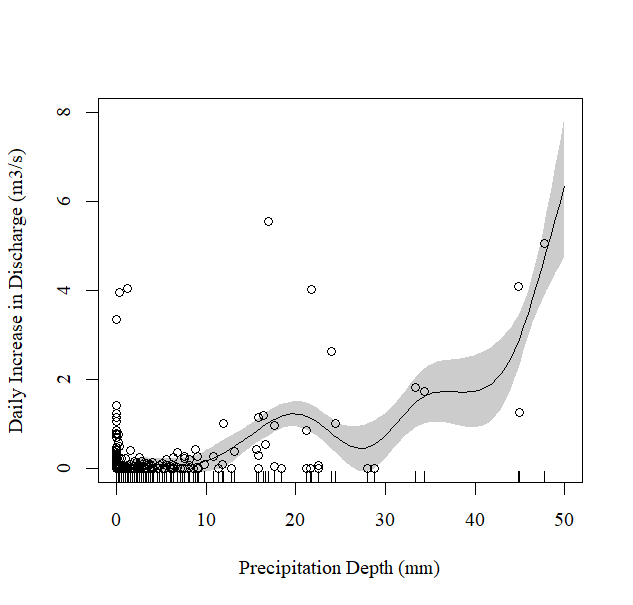
Figure 1: Control GAM Model for Relationship Between Precipitation Depth (mm) and the Daily Increase in Stream Discharge (m3/s)
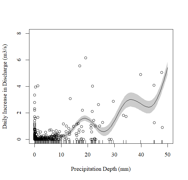
Figure 2: Treatment GAM Model for Relationship Between Precipitation Depth (mm) and the Daily Increase in Stream Discharge (m3/s)
I now want to determine the model equations for each of my GAM models to see if the effect size of precipitation depth on the daily increase in stream discharge is reduced in the post-treatment scenario (compared to the pre-treatment scenario).
Does anyone have any advice on how to determine model equations for my GAM models? I was looking online but cannot find any answers relevant to what I am attempting to accomplish.
TIA