Determine Statistical Difference Between Two Groups

brant · February 22, 2025, 4:44pm

Hi, I am having trouble calculating a p-value to show statistical differences between sites for an upcoming conference poster. I have suspended solids concentrations for six different sites and created a graph of the mean concentrations for each site (as shown below)

The sample sizes for Inflow 1, Outflow 1, Inflow 2, Outflow 2, Inflow 3, and Outflow 3 are 25, 25, 12, 12, 14, 14, respectively.

I am trying to determine if:

Inflow 1 (n = 25) is statistically different from Outflow 1 (n = 25)
Inflow 2 (n = 12) is statistically different from Outflow 2 (n = 12)
Inflow 3 (n = 14) is statistically different from Outflow 3 (n = 14)

I tried running a Wilcoxon rank-sum test to compare each group, but I am getting the following outputs:

> test_result <- wilcox.test(inflow1, outflow1)
> print(test_result)

	Wilcoxon rank sum exact test

data:  inflow1 and outflow1
W = 408, p-value = 0.06495
alternative hypothesis: true location shift is not equal to 0

Error in wilcox.test.default(inflow2, outflow2, exact = FALSE) : 
  not enough (non-missing) 'x' observations
> print(test_result)# p = 0.06

	Wilcoxon rank sum exact test

data:  inflow1 and outflow1
W = 408, p-value = 0.06495
alternative hypothesis: true location shift is not equal to 0

> test_result <- wilcox.test(inflow3, outflow3, exact = FALSE) # Typically want at least 10 observations per group 
Error in wilcox.test.default(inflow3, outflow3, exact = FALSE) : 
  not enough (non-missing) 'x' observations
> print(test_result)# p = 0.06

	Wilcoxon rank sum exact test

data:  inflow1 and outflow1
W = 408, p-value = 0.06495
alternative hypothesis: true location shift is not equal to 0

I have a few problems here:

When running the Wilcoxon rank-sum test for inflow1 and outflow1, I am getting a p-value of 0.06495. I definitely expected the difference to be significant.
When running the Wilcoxin rank-sum test for inflow2 and outflow 2, I am getting the error shown below:

> test_result <- wilcox.test(inflow2, outflow2, exact = FALSE)  
Error in wilcox.test.default(inflow2, outflow2, exact = FALSE) : 
  not enough (non-missing) 'x' observations

It appears as if my error is due to having too small of a sample size (n = 25 for inflow1 and outflow1, n = 12 for inflow2 and outflow2, and n = 14 for inflow3 and outflow3). Does anyone have any advice as to how to determine:

Statistical difference between inflow1 and outflow1
Statistical difference between inflow2 and outflow2
Statistical difference between inflow3 and outflow3.

For every sample set collected the outflow concentrations were approximately half of the inflow concentrations, so I have a hard time believing that they wouldn't be statistically different. I want to be able to show the p-values for my conference poster though.

FJCC · February 22, 2025, 5:07pm

Can you post your data ? The output of

dput(inflow2)
dput(outflow2)

would allow others to replicate your test.

jrkrideau · February 22, 2025, 5:59pm

I second FJCC request but if your data is in a data.frame or tibble, it probable would be better to supply the entire dataset.

Do dput(mydata) where "mydata" is the name of your dataset. For really large datasets probably dput(head(mydata, 100)) will do. Paste the output between
```

```

Am I correct that Inflow1 and Outflow1 is the input and output from a single process?

May I ask why you are using a wilcox.test?

brant · February 22, 2025, 8:57pm

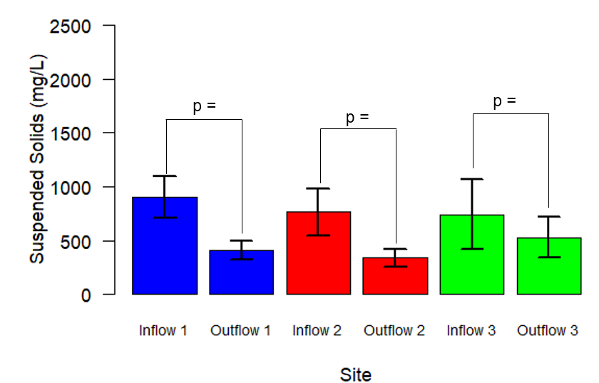
Thank you. I just posted my data below. Note that the site names in my raw data correspond to street names, and are thus different than what is shown in the graph. "Inflow 1" = "Hinton Inflow Front Cell", "Outflow 1" = "Hinton Outflow", "Inflow 2" = "Cuyler and Dewe Inflow", "Outflow 2" = "Cuyler and Dewe Outflow", "Inflow 3" = "Cuyler and Current Inflow", and "Outflow 3" = "Cuyler and Current Outflow"

dput(head(rainfall,100))
structure(list(Rainfall.Number = c(1L, 1L, 1L, 1L, 1L, 1L, 1L, 
1L, 1L, 2L, 2L, 2L, 2L, 2L, 2L, 2L, 2L, 2L, 2L, 3L, 3L, 4L, 4L, 
4L, 4L, 4L, 4L, 4L, 4L, 4L, 4L, 4L, 5L, 5L, 5L, 5L, 5L, 5L, 5L, 
5L, 5L, 5L, 6L, 6L, 6L, 6L, 6L, 6L, 6L, 6L, 6L, 6L, 6L, 7L, 7L, 
7L, 7L, 7L, 7L, 7L, 8L, 8L, 8L, 8L, 8L, 8L, 8L, 8L, 8L, 8L, 8L, 
8L, 9L, 9L, 9L, 9L, 9L, 9L, 9L, 9L, 9L, 10L, 10L, 10L, 10L, 10L, 
10L, 10L, 10L, 10L, 11L, 11L, 11L, 11L, 11L, 11L, 11L, 12L, 12L, 
12L), Date = c("2022-08-05", "2022-08-05", "2022-08-05", "2022-08-05", 
"2022-08-05", "2022-08-05", "2022-08-05", "2022-08-05", "2022-08-05", 
"2022-08-18", "2022-08-18", "2022-08-18", "2022-08-18", "2022-08-18", 
"2022-08-18", "2022-08-18", "2022-08-18", "2022-08-18", "2022-08-18", 
"2022-08-23", "2022-08-23", "2022-09-09", "2022-09-09", "2022-09-09", 
"2022-09-09", "2022-09-09", "2022-09-09", "2022-09-09", "2022-09-09", 
"2022-09-09", "2022-09-09", "2022-09-09", "2022-09-25", "2022-09-25", 
"2022-09-25", "2022-09-25", "2022-09-25", "2022-09-25", "2022-09-25", 
"2022-09-25", "2022-09-25", "2022-09-25", "2022-10-12", "2022-10-12", 
"2022-10-12", "2022-10-12", "2022-10-12", "2022-10-12", "2022-10-12", 
"2022-10-12", "2022-10-12", "2022-10-12", "2022-10-12", "2022-11-06", 
"2022-11-06", "2022-11-06", "2022-11-06", "2022-11-06", "2022-11-06", 
"2022-11-06", "2023-04-29", "2023-04-29", "2023-04-29", "2023-04-29", 
"2023-04-29", "2023-04-29", "2023-04-29", "2023-04-29", "2023-04-29", 
"2023-04-29", "2023-04-29", "2023-04-29", "2023-05-19", "2023-05-19", 
"2023-05-19", "2023-05-19", "2023-05-19", "2023-05-19", "2023-05-19", 
"2023-05-19", "2023-05-19", "2023-06-24", "2023-06-24", "2023-06-24", 
"2023-06-24", "2023-06-24", "2023-06-24", "2023-06-24", "2023-06-24", 
"2023-06-24", "2023-06-29", "2023-06-29", "2023-06-29", "2023-06-29", 
"2023-06-29", "2023-06-29", "2023-06-29", "2023-07-09", "2023-07-09", 
"2023-07-09"), Site = c("Hinton Upstream", "Hinton Inflow Front Cell", 
"Hinton Outflow", "Hinton Downstream", "Blanchard Upstream", 
"Blanchard Inflow", "Blanchard Downstream", "Cuyler and Dewe Inflow", 
"Cuyler and Dewe Outflow", "Hinton Upstream", "Hinton Inflow Front Cell", 
"Hinton Inflow Back Cell", "Hinton Outflow", "Hinton Downstream", 
"Blanchard Upstream", "Blanchard Inflow", "Blanchard Downstream", 
"Cuyler and Current Inflow", "Cuyler and Current Outflow", "Cuyler and Current Inflow", 
"Cuyler and Current Outflow", "Hinton Upstream", "Hinton Inflow Front Cell", 
"Hinton Outflow", "Hinton Downstream", "Blanchard Upstream", 
"Blanchard Inflow", "Blanchard Downstream", "Cuyler and Dewe Inflow", 
"Cuyler and Dewe Outflow", "Cuyler and Current Inflow", "Cuyler and Current Outflow", 
"Hinton Upstream", "Hinton Inflow Front Cell", "Hinton Inflow Back Cell", 
"Hinton Outflow", "Hinton Downstream", "Blanchard Upstream", 
"Blanchard Inflow", "Blanchard Downstream", "Cuyler and Current Inflow", 
"Cuyler and Current Outflow", "Hinton Upstream", "Hinton Inflow Front Cell", 
"Hinton Outflow", "Hinton Downstream", "Blanchard Upstream", 
"Blanchard Inflow", "Blanchard Downstream", "Cuyler and Dewe Inflow", 
"Cuyler and Dewe Outflow", "Cuyler and Current Inflow", "Cuyler and Current Outflow", 
"Hinton Upstream", "Hinton Inflow Front Cell", "Hinton Outflow", 
"Hinton Downstream", "Blanchard Upstream", "Blanchard Inflow", 
"Blanchard Downstream", "Blanchard Upstream", "Blanchard Inflow", 
"Blanchard Downstream", "Hinton Upstream", "Hinton Inflow Front Cell", 
"Hinton Inflow Back Cell", "Hinton Outflow", "Hinton Downstream", 
"Cuyler and Dewe Inflow", "Cuyler and Dewe Outflow", "Cuyler and Current Inflow", 
"Cuyler and Current Outflow", "Blanchard Upstream", "Blanchard Inflow", 
"Blanchard Downstream", "Hinton Upstream", "Hinton Inflow Front Cell", 
"Hinton Outflow", "Hinton Downstream", "Cuyler and Current Inflow", 
"Cuyler and Current Outflow", "Blanchard Upstream", "Blanchard Inflow", 
"Blanchard Downstream", "Hinton Upstream", "Hinton Inflow Front Cell", 
"Hinton Outflow", "Hinton Downstream", "Cuyler and Dewe Inflow", 
"Cuyler and Dewe Outflow", "Blanchard Upstream", "Blanchard Inflow", 
"Blanchard Downstream", "Hinton Upstream", "Hinton Inflow Front Cell", 
"Hinton Outflow", "Hinton Downstream", "Blanchard Upstream", 
"Blanchard Inflow", "Blanchard Downstream"), pH = c(7.84, 6.24, 
7.51, 8.25, 8.07, 7.35, 8.11, 8.52, 7.85, 8.01, 7.76, 7.08, 7.51, 
8.23, 7.77, 7.09, 7.78, 7.32, 7.04, 6.98, 7.22, 8.27, 7.71, 6.99, 
7.88, 8.09, 7.39, 7.96, 8.79, 7.58, 7.22, 6.95, 7.81, 7.41, 7.7, 
7.81, 7.68, 7.88, 7.25, 7.82, 7.31, 6.92, 8.05, 6.93, 7.96, 8.03, 
8, 7.31, 7.66, 8.05, 7.65, 7.25, 7, 7.9, 6.68, 6.78, 7.86, 8.09, 
6.69, 7.85, 7.64, 7.86, 7.57, 7.48, 7.82, 7.72, 7.4, 7.74, 8.04, 
7.58, 7.96, 7.72, 7.73, 7.27, 7.56, 7.68, 6.41, 7.1, 7.78, 6.96, 
6.65, 7.6, 6.67, 7.99, 7.88, 5.3, 6.97, 7.67, 7.62, 7.37, 7.72, 
6.53, 8.03, 8.04, 6.88, 7.06, 8.04, 7.96, 6.07, 7.66), TDS = c(224L, 
39L, 165L, 230L, 231L, 25L, 250L, 45L, 42L, 269L, 20L, 44L, 223L, 
254L, 170L, 48L, 155L, 20L, 191L, 35L, 188L, 379L, 66L, 99L, 
283L, 312L, 62L, 271L, 44L, 47L, 13L, 87L, 219L, 16L, 228L, 204L, 
213L, 218L, 19L, 231L, 22L, 197L, 282L, 53L, 193L, 277L, 246L, 
27L, 241L, 59L, 61L, 24L, 175L, 210L, 47L, 102L, 201L, 232L, 
36L, 211L, 209L, 47L, 182L, 191L, 65L, 166L, 273L, 180L, 50L, 
199L, 39L, 49L, 148L, 63L, 153L, 140L, 137L, 159L, 147L, 33L, 
410L, 251L, 35L, 268L, 255L, 127L, 150L, 255L, 77L, 150L, 245L, 
39L, 243L, 461L, 82L, 140L, 238L, 293L, 47L, 249L), Ec = c(447L, 
78L, 330L, 460L, 463L, 51L, 500L, 90L, 85L, 536L, 41L, 88L, 446L, 
510L, 340L, 96L, 310L, 40L, 382L, 71L, 377L, 782L, 133L, 199L, 
567L, 625L, 124L, 540L, 88L, 93L, 26L, 175L, 438L, 32L, 456L, 
408L, 426L, 436L, 38L, 462L, 44L, 395L, 568L, 106L, 386L, 554L, 
492L, 55L, 481L, 118L, 123L, 47L, 350L, 421L, 95L, 204L, 401L, 
512L, 72L, 422L, 417L, 95L, 364L, 383L, 131L, 338L, 545L, 360L, 
99L, 398L, 77L, 100L, 297L, 125L, 308L, 281L, 279L, 318L, 293L, 
66L, 819L, 501L, 70L, 536L, 510L, 254L, 300L, 511L, 154L, 301L, 
490L, 77L, 487L, 231L, 164L, 280L, 475L, 586L, 95L, 497L), Turbidity..NTU. = c(1.64, 
7.25, 5.63, 2.06, 3.08, 5.62, 3.29, 11.1, 3.95, 7.15, 12.9, 7.71, 
7.5, 7.1, 21.4, 12.5, 19.6, 3.84, 3.11, 81.7, 20.6, 5.9, 47.2, 
63.8, 7.44, 2.92, 9.21, 2.21, 7.31, 6.12, 29.3, 11.6, 6.9, 4.8, 
7, 7.11, 9.26, 3.93, 7.28, 4.01, 8.11, 3.59, 6.64, 7.12, 0.25, 
5.32, 2.43, 12.5, 6.25, 28.1, 4.95, 4.32, 8.78, 6.42, 27.1, 24.8, 
7.21, 3.99, 12.2, 0.7, 16.1, 37, 14, 8.56, 60.6, 7.41, 16.5, 
13.2, 98, 43.8, 31.6, 9.42, 12.1, 60.4, 14.9, 34.2, 94, 66.4, 
22.1, 55.5, 6.55, 34.4, 4.87, 16.4, 4.07, 644, 25.9, 4.69, 32.9, 
27.8, 52.8, 37.9, 53.5, 17.8, 91.7, 26.1, 63, 36.2, 30, 9.07), 
    TSS..g.L. = c(NA, NA, NA, NA, NA, NA, NA, NA, NA, 8.408, 
    8.794, 8.794, 8.898, 8.97, 9.67, 8.646, 4.32, 8.52, 8.96, 
    9.1, 8.85, 8.92, 9.38, 8.9, 8.27, 8.19, 8.59, 8.4, 8.64, 
    8.5, 8.5, 4.23, 8.59, 8.86, 8.66, 7.98, 8.2, 8.67, 8.55, 
    8.68, 4.21, 4.48, 4.193, 4.866, 4.28, 4.44, 4.29, 4.24, 4.57, 
    4.38, 4.21, 4.46, 4.54, 6.2, 5.124, 4.88, 6, 6, 7.2, 6.02, 
    123, 105, 95, 109, 250, 70.59, 91.95, 117.65, 313.87, 237.7, 
    98.16, 57.43, 66.797, 248.7, 47.964, 73.333, 484.63, 197.909, 
    851.33, 4449.04, 2487.91, 127.17, 431.37, 241.76, 177.78, 
    1107.53, 196.26, 172.73, 233.01, 162.16, 282.21, 482.35, 
    401.96, 120.97, 821.92, 367.92, 2365.52, 192.1, 299.1, 82
    ), DOC..mg.L. = c(NA, NA, NA, NA, NA, NA, NA, NA, NA, 16.65, 
    10.65, 14.73, 14.23, 16.05, 9.114, 21.52, 11.7, 25.6, 16.19, 
    18.37, 10.04, 11.52, 14.8, 20.12, 18, 12.27, 23.27, 15.02, 
    25.01, 27.82, 14.2, 9.55, 17.88, 8.045, 16.73, 14.78, 18.15, 
    18.34, 10.75, 17.67, 13.8, 9.05, 14.97, 23.41, 7.97, 12.75, 
    12.45, 11.86, 12.63, 7.92, 10.61, 15.7, 7.9, 13.57, 17.73, 
    19.35, 14.36, 13.08, 28.47, 13.83, 14.95, 13.49, 14.44, 15.2, 
    17.3, 9.759, 12.16, 14.71, 8.33, 10.02, 10.25, 7.567, 15.89, 
    31.11, 17.56, 15.45, 17.45, 16.01, 15.73, 24.65, 9.027, 18.34, 
    26.98, 17.87, 11.88, 16.56, 31.58, 11.81, 15.9, 18.9, 15.79, 
    21.12, 12.01, 12.1, 16.35, 13.73, 14.11, 15.88, 29.54, 14.21
    ), Ammonia = c("0.78", "4.32", "0.54", "0.78", "0.43", "1.3", 
    "0.23", "0.24", "0.36", "0.92", "0.43", "0.6", "0.48", "0.31", 
    "1.8", "3.44", "2.11", "0.34", "0.3", "0.78", "0.23", "2.52", 
    "1.24", "1.74", "0.48", "0.35", "0.54", "0.43", "3.36", "0.31", 
    "0.47", "0.21", "0.35", "0.47", "0.13", "0.56", "0.28", "0.44", 
    "0.47", "0.39", "0.24", "0.2", "1.42", "0.69", "0.39", "1.49", 
    "0.36", "1.06", "0.84", "1.58", "0.73", "1.3", "0.78", "1.88", 
    "0.91", "0.32", "1.42", "0.64", "0.37", "0.48", "0.74", "1.76", 
    "0.29", "0.27", "3", "7.84", "0.68", "0.18", "0.77", "0.54", 
    "0.85", "1", "1.82", "0.54", "0.18", "0.67", "0.76", "0.66", 
    "0.89", "1.02", "0.57", "0.95", "0.79", "0.96", "0.37", "0.85", 
    "0.52", "0.37", "0.64", "0.79", "0.82", "0.96", "2", "0.29", 
    "1.42", "0.26", "0.65", "1.34", "1.5", "1.32"), Nitrate = c(0.172, 
    0.161, 0.155, 0.434, 0.405, 0.124, 0.399, 0.131, 0.178, 1.01, 
    0.138, 0.845, 0.5, 0.6, 0.25, 0.214, 0.403, 0.15, 0.72, 0.54, 
    0.61, 0.341, 0.44, 0.329, 0.99, 1.01, 1.327, 1.29, 0.985, 
    1.67, 0.03, 0.276, 0.15, 0.308, 0.605, 0.299, 0.337, 0.755, 
    0.144, 0.532, 0.091, 0.135, 0.301, 0.052, 0.194, 0.227, 0.388, 
    0.291, 0.239, 0.132, 0.484, 0.164, 0.139, 0.349, 0.379, 0.094, 
    0.281, 0.885, 0.077, 0.069, 0.51, 0.062, 0.227, 0.254, 0.001, 
    0.246, 0.095, 0.34, 0, 0.028, 0.13, 0.299, 0.304, 0.015, 
    0.171, 0.198, 0.349, 0.222, 0.195, 0.185, 0.379, 0.161, 0.165, 
    0.161, 0.293, 0.68, 0.125, 0.066, 0.149, 0.77, 0.319, 0.141, 
    0.255, 0.178, 0.54, 0.12, 0.177, 0.229, 0.073, 0.228), Nitrite = c(0.004, 
    0.03, 0.013, 0.029, 0.007, 0.016, 0.007, 0.007, 0.009, 0.004, 
    0.006, 0.005, 0.055, 0.059, 0.009, 0.024, 0.001, 0.007, 0.004, 
    0.01, 0.01, 0.035, 0.01, 0.066, 0.021, 0.016, 0.015, 0.02, 
    0.042, 0.011, 0.008, 0.008, 0.018, 0.009, 0.03, 0.008, 0.012, 
    0.029, 0.008, 0.037, 0.013, 0.008, 0.01, 0.001, 0.019, 0.016, 
    0.008, 0.021, 0.006, 0.017, 0.017, 0.016, 0.015, 0.006, 0.001, 
    0.001, 0.007, 0.006, 0.003, 0.002, 0.008, 0.001, 0.008, 0.064, 
    0.001, 0.009, 0.001, 0.01, 0, 0, 0.002, 0.007, 0.008, 0.05, 
    0.032, 0.008, 0.027, 0.009, 0.019, 0.008, 0.008, 0.012, 0.027, 
    0.041, 0.047, 0.036, 0.033, 0.019, 0.04, 0.019, 0.016, 0.004, 
    0.042, 0.014, 0.84, 0.019, 0.028, 0.015, 0.001, 0.015), Phosphate = c(0.14, 
    0.23, 0.11, 0.13, 0.01, 0.14, 0.01, 0.15, 0.16, 0.01, 0.22, 
    0.29, 0.54, 0.16, 0.36, 0.18, 0.39, 0.16, 0.15, 0.81, 1.76, 
    0.17, 0.47, 0.53, 0.17, 0.79, 0.93, 0.48, 0.34, 0.63, 0.29, 
    0.22, 0.17, 0.06, 0.11, 0.13, 0.15, 0.13, 0.01, 0.13, 0.19, 
    0.31, 0.01, 0.18, 0.32, 0.19, 0.12, 0.29, 0.15, 0.3, 0.91, 
    0.18, 0.72, 0.18, 0.16, 0.22, 0.13, 0.1, 0.77, 0.15, 0.04, 
    0.1, 0.06, 0.16, 0.05, 0.38, 0.42, 0.35, 0.43, 0.21, 0.51, 
    0.38, 0.26, 0.18, 0.22, 0.13, 0.32, 0.22, 0.11, 0.27, 0.01, 
    0.17, 0.01, 0.01, 0.07, 0.32, 0.24, 0.63, 0.25, 3.5, 0.36, 
    0.84, 0.2, 0.1, 2.2, 0.26, 0.67, 0.33, 0, 0.32), Zinc = c(0.67, 
    0.82, 0.33, 0.08, 0.35, 0.29, 0.03, 0.09, 0.1, 1.62, 0.24, 
    0.05, 0.21, 0.59, 0.28, 0.08, 3.92, 0.63, 1.21, 0.04, 0.26, 
    0.97, 0.11, 0.13, 0.47, 0.18, 0.63, 0.63, 0.33, 0.25, 0.2, 
    0.23, 0.38, 0.17, 0.11, 0.32, 0.23, 0.19, 0.15, 0.27, 0.55, 
    0.3, 2.44, 0.31, 0.16, 2.13, 1.02, 0.14, 1.06, 0.15, 1.05, 
    0.3, 0.21, 0.15, 0.13, 0.26, 0.14, 0.56, 0.4, 0.46, 0.18, 
    0.4, 0.26, 0.45, 0.01, 0.29, 0.22, 0.45, 0.25, 0.63, 0.26, 
    0.13, 0.19, 0.7, 0.76, 0.09, 0.73, 0.22, 0.13, 0.23, 0.21, 
    0.01, 0.04, 0.01, 0.01, 1.27, 0.05, 0.01, 1.01, 0.17, 1.14, 
    1.09, 0.4, 0.61, 1.72, 0.74, 0.56, 0.6, 0.04, 0.6), Iron = c(0.17, 
    0.14, 0.09, 0.12, 0.28, 0.06, 0.32, 0.04, 0.17, 0.1, 0.05, 
    0.04, 0.17, 0.14, 0.17, 0.01, 0.11, 0.06, 0.18, 0.01, 0.17, 
    0.11, 0.25, 0.53, 0.12, 0.15, 0.33, 0.23, 0.14, 0.07, 0.07, 
    0.01, 0.13, 0.04, 0.07, 0.07, 0.21, 0.27, 0.14, 0.15, 0.11, 
    0.05, 0.08, 1, 0.06, 0.53, 0.1, 0.04, 0.09, 0.07, 0.21, 0.04, 
    0.03, 0.28, 0.28, 0.37, 0.25, 0.24, 0.05, 0.11, 0.09, 0.31, 
    0.06, 0.22, 0.16, 0.08, 0.07, 0.42, 0.11, 0.01, 0.28, 0.01, 
    0.11, 0.27, 0.08, 0.06, 0.17, 0.14, 0.17, 0.01, 0.02, 0.01, 
    0.01, 0.01, 0.01, 0.37, 0.24, 0.01, 0.28, 0.06, 0.22, 0.12, 
    0.09, 0.11, 0.28, 0.21, 0.09, 0.19, 0.04, 0.18), Chloride = c(16, 
    14, 3.4, 7.4, 11.5, 0, 8.3, 2.7, 22, 16, 30, 21, 8.4, 16, 
    15.5, 14, 16, 8, 15, 9.3, 19.5, 13, 11.5, 11.5, 17.5, 10.5, 
    4.7, 16, 13, 1.4, 29, 18, 9.1, 21, 4.9, 25, 5.7, 5.9, 10, 
    6.2, 17.5, 7.2, 34, 0.01, 7.7, 14, 6.9, 2, 11, 13.5, 10.5, 
    25, 18, 5.6, 11, 3.3, 5.7, 6.3, 5.3, 8.2, 21, 11.5, 23, 7.8, 
    0.7, 4.7, 21.5, 8.2, 0.01, 10.5, 15, 21, 20.5, 4.4, 4.5, 
    3.3, 0.01, 6.2, 3.4, 10, 18, 0.5, 0, 5, 2.8, 0, 3.2, 3.7, 
    0, 0, 13.5, 10.5, 9.2, 15, 18.5, 12.5, 11.5, 11, 12.5, 11
    )), row.names = c(NA, 100L), class = "data.frame")

brant · February 22, 2025, 9:06pm

@jrkrideau Yes, Inflow1 and Outflow 1 are the input and output from a single process, Inflow 2 and Outflow 2 are the input and output from another process, and Inflow 3 and Outflow 3 are the input and output from a third process. I was using a wilcox.test because my sample size is relatively small (n = 25 for Inflow 1 and Outflow 1, n = 12 for Inflow 2 and Outflow 2, and n = 14 for Inflow 3 and Outflow 3). It is expected that for each process, the outflow concentrations will be lower than the inflow concentrations, but I want to test the statistical significance of this. I am open to any suggestions if there is a better way to do this than a wilcox.test. It doesn't make much difference to me as long as i can accurately test statistical differences between sites and assign a p-value to my graph.

brant · February 22, 2025, 9:21pm

I am ultimately trying to add p-values to the graph below for one of my conference presentations next month. I am open to any suggestions on tests to use as long as they will help me test for statistical difference between these bars.

FJCC · February 22, 2025, 9:55pm

Thanks for posting the data. I'm confused by it. I loaded it into a data frame named DF and used table() to count the occurrences of each Site.

 table(DF$Site)

      Blanchard Downstream           Blanchard Inflow         Blanchard Upstream  Cuyler and Current Inflow 
                        11                         11                         11                          7 
Cuyler and Current Outflow     Cuyler and Dewe Inflow    Cuyler and Dewe Outflow          Hinton Downstream 
                         7                          5                          5                         10 
   Hinton Inflow Back Cell   Hinton Inflow Front Cell             Hinton Outflow            Hinton Upstream 
                         3                         10                         10                         10

The sites you list have 10, 5 and 7 samples, not 25, 12, and 14. Also, it is not clear which column you have plotted. Since your plot labels the y axis Suspended Solids, I guess TSS..g.L, but summarizing that column by Site gives values very different from you plot.

  Site        Avg
  <chr>     <dbl>
1 Inflow 1  300. 
2 Inflow 2  140. 
3 Inflow 3  655. 
4 Outflow 1  98.8
5 Outflow 2 103. 
6 Outflow 3 368.

Please explain how your data maps to your plot and quoted sample numbers.

brant · February 22, 2025, 10:25pm

@FJCC. Sorry for the confusion. Posit would not allow me to upload all of the occurrences due to character restrictions on this forum. My full data has samples sizes of 25, 12 and 14, but in my dput() function I only included the first 100 records as I have a fairly large dataset. It appears that the first 100 records provides 10, 5, and 7 samples, while my full dataset has 25, 12, and 14 samples. Posit only allows us to pose up to 32000 characters in this forum. My full dataset has 32184 characters.

Likewise the first 100 records is only a small snapshot of my data and does not capture seasonality (i.e., suspended concentrations are higher in spring, and my dput() data provided fall data). This is likely why you have very different values than what I plotted.

In terms of how my data maps to my plot:

Hinton Inflow Front Cell = Inflow 1
Hinton Outflow = Outflow 1
Cuyler and Dewe Inflow = Inflow 2
Cuyler and Dewe Outflow = Outflow 2
Cuyler and Current Inflow = Inflow 3
Cuyler and Current Outflow = Outflow 3

I am plotting the column TSS..g.L. Sorry for the confusion.

FJCC · February 23, 2025, 5:51am

Here is an example of running the wilcox.test() on your suspended solid values without getting an error. I deleted the unnecessary columns from your data frame to simplify the example.

library(tidyverse)
DF <- structure(list(Rainfall.Number = c(1L, 1L, 1L, 1L, 1L, 1L, 1L, 
                                         1L, 1L, 2L, 2L, 2L, 2L, 2L, 2L, 2L, 2L, 2L, 2L, 3L, 3L, 4L, 4L, 
                                         4L, 4L, 4L, 4L, 4L, 4L, 4L, 4L, 4L, 5L, 5L, 5L, 5L, 5L, 5L, 5L, 
                                         5L, 5L, 5L, 6L, 6L, 6L, 6L, 6L, 6L, 6L, 6L, 6L, 6L, 6L, 7L, 7L, 
                                         7L, 7L, 7L, 7L, 7L, 8L, 8L, 8L, 8L, 8L, 8L, 8L, 8L, 8L, 8L, 8L, 
                                         8L, 9L, 9L, 9L, 9L, 9L, 9L, 9L, 9L, 9L, 10L, 10L, 10L, 10L, 10L, 
                                         10L, 10L, 10L, 10L, 11L, 11L, 11L, 11L, 11L, 11L, 11L, 12L, 12L, 
                                         12L), Date = c("2022-08-05", "2022-08-05", "2022-08-05", "2022-08-05", 
                                                        "2022-08-05", "2022-08-05", "2022-08-05", "2022-08-05", "2022-08-05", 
                                                        "2022-08-18", "2022-08-18", "2022-08-18", "2022-08-18", "2022-08-18", 
                                                        "2022-08-18", "2022-08-18", "2022-08-18", "2022-08-18", "2022-08-18", 
                                                        "2022-08-23", "2022-08-23", "2022-09-09", "2022-09-09", "2022-09-09", 
                                                        "2022-09-09", "2022-09-09", "2022-09-09", "2022-09-09", "2022-09-09", 
                                                        "2022-09-09", "2022-09-09", "2022-09-09", "2022-09-25", "2022-09-25", 
                                                        "2022-09-25", "2022-09-25", "2022-09-25", "2022-09-25", "2022-09-25", 
                                                        "2022-09-25", "2022-09-25", "2022-09-25", "2022-10-12", "2022-10-12", 
                                                        "2022-10-12", "2022-10-12", "2022-10-12", "2022-10-12", "2022-10-12", 
                                                        "2022-10-12", "2022-10-12", "2022-10-12", "2022-10-12", "2022-11-06", 
                                                        "2022-11-06", "2022-11-06", "2022-11-06", "2022-11-06", "2022-11-06", 
                                                        "2022-11-06", "2023-04-29", "2023-04-29", "2023-04-29", "2023-04-29", 
                                                        "2023-04-29", "2023-04-29", "2023-04-29", "2023-04-29", "2023-04-29", 
                                                        "2023-04-29", "2023-04-29", "2023-04-29", "2023-05-19", "2023-05-19", 
                                                        "2023-05-19", "2023-05-19", "2023-05-19", "2023-05-19", "2023-05-19", 
                                                        "2023-05-19", "2023-05-19", "2023-06-24", "2023-06-24", "2023-06-24", 
                                                        "2023-06-24", "2023-06-24", "2023-06-24", "2023-06-24", "2023-06-24", 
                                                        "2023-06-24", "2023-06-29", "2023-06-29", "2023-06-29", "2023-06-29", 
                                                        "2023-06-29", "2023-06-29", "2023-06-29", "2023-07-09", "2023-07-09", 
                                                        "2023-07-09"), 
                     Site = c("Hinton Upstream", "Hinton Inflow Front Cell", 
                              "Hinton Outflow", "Hinton Downstream", "Blanchard Upstream", 
                              "Blanchard Inflow", "Blanchard Downstream", "Cuyler and Dewe Inflow", 
                              "Cuyler and Dewe Outflow", "Hinton Upstream", "Hinton Inflow Front Cell", 
                              "Hinton Inflow Back Cell", "Hinton Outflow", "Hinton Downstream", 
                              "Blanchard Upstream", "Blanchard Inflow", "Blanchard Downstream", 
                              "Cuyler and Current Inflow", "Cuyler and Current Outflow", "Cuyler and Current Inflow", 
                              "Cuyler and Current Outflow", "Hinton Upstream", "Hinton Inflow Front Cell", 
                              "Hinton Outflow", "Hinton Downstream", "Blanchard Upstream", 
                              "Blanchard Inflow", "Blanchard Downstream", "Cuyler and Dewe Inflow", 
                              "Cuyler and Dewe Outflow", "Cuyler and Current Inflow", "Cuyler and Current Outflow", 
                              "Hinton Upstream", "Hinton Inflow Front Cell", "Hinton Inflow Back Cell", 
                              "Hinton Outflow", "Hinton Downstream", "Blanchard Upstream", 
                              "Blanchard Inflow", "Blanchard Downstream", "Cuyler and Current Inflow", 
                              "Cuyler and Current Outflow", "Hinton Upstream", "Hinton Inflow Front Cell", 
                              "Hinton Outflow", "Hinton Downstream", "Blanchard Upstream", 
                              "Blanchard Inflow", "Blanchard Downstream", "Cuyler and Dewe Inflow", 
                              "Cuyler and Dewe Outflow", "Cuyler and Current Inflow", "Cuyler and Current Outflow", 
                              "Hinton Upstream", "Hinton Inflow Front Cell", "Hinton Outflow", 
                              "Hinton Downstream", "Blanchard Upstream", "Blanchard Inflow", 
                              "Blanchard Downstream", "Blanchard Upstream", "Blanchard Inflow", 
                              "Blanchard Downstream", "Hinton Upstream", "Hinton Inflow Front Cell", 
                              "Hinton Inflow Back Cell", "Hinton Outflow", "Hinton Downstream", 
                              "Cuyler and Dewe Inflow", "Cuyler and Dewe Outflow", "Cuyler and Current Inflow", 
                              "Cuyler and Current Outflow", "Blanchard Upstream", "Blanchard Inflow", 
                              "Blanchard Downstream", "Hinton Upstream", "Hinton Inflow Front Cell", 
                              "Hinton Outflow", "Hinton Downstream", "Cuyler and Current Inflow", 
                              "Cuyler and Current Outflow", "Blanchard Upstream", "Blanchard Inflow", 
                              "Blanchard Downstream", "Hinton Upstream", "Hinton Inflow Front Cell", 
                              "Hinton Outflow", "Hinton Downstream", "Cuyler and Dewe Inflow", 
                              "Cuyler and Dewe Outflow", "Blanchard Upstream", "Blanchard Inflow", 
                              "Blanchard Downstream", "Hinton Upstream", "Hinton Inflow Front Cell", 
                              "Hinton Outflow", "Hinton Downstream", "Blanchard Upstream", 
                              "Blanchard Inflow", "Blanchard Downstream"), 
                     TSS..g.L. = c(NA, NA, NA, NA, NA, NA, NA, NA, NA, 8.408, 
                                   8.794, 8.794, 8.898, 8.97, 9.67, 8.646, 4.32, 8.52, 8.96, 
                                   9.1, 8.85, 8.92, 9.38, 8.9, 8.27, 8.19, 8.59, 8.4, 8.64, 
                                   8.5, 8.5, 4.23, 8.59, 8.86, 8.66, 7.98, 8.2, 8.67, 8.55, 
                                   8.68, 4.21, 4.48, 4.193, 4.866, 4.28, 4.44, 4.29, 4.24, 4.57, 
                                   4.38, 4.21, 4.46, 4.54, 6.2, 5.124, 4.88, 6, 6, 7.2, 6.02, 
                                   123, 105, 95, 109, 250, 70.59, 91.95, 117.65, 313.87, 237.7, 
                                   98.16, 57.43, 66.797, 248.7, 47.964, 73.333, 484.63, 197.909, 
                                   851.33, 4449.04, 2487.91, 127.17, 431.37, 241.76, 177.78, 
                                   1107.53, 196.26, 172.73, 233.01, 162.16, 282.21, 482.35, 
                                   401.96, 120.97, 821.92, 367.92, 2365.52, 192.1, 299.1, 82
                     )), row.names = c(NA, 100L), class = "data.frame")




DFnew <- DF |> mutate(Site = case_when(
Site ==  'Hinton Inflow Front Cell' ~ 'Inflow_1',
Site == 'Hinton Outflow' ~ 'Outflow_1',
Site == 'Cuyler and Dewe Inflow' ~ 'Inflow_2',
Site == 'Cuyler and Dewe Outflow' ~ 'Outflow_2',
Site == 'Cuyler and Current Inflow' ~ 'Inflow_3',
Site == 'Cuyler and Current Outflow' ~ 'Outflow_3',
TRUE ~ 'Not Appl'
)) |> filter(Site != 'Not Appl') |> 
  select(Rainfall.Number, Site, TSS..g.L.) |> 
  pivot_wider(names_from = Site, values_from = 'TSS..g.L.')

wilcox.test(DFnew$Inflow_1, DFnew$Outflow_1, data = tmp)
#> 
#>  Wilcoxon rank sum exact test
#> 
#> data:  DFnew$Inflow_1 and DFnew$Outflow_1
#> W = 49, p-value = 0.4894
#> alternative hypothesis: true location shift is not equal to 0
wilcox.test(DFnew$Inflow_2, DFnew$Outflow_2, data = tmp)
#> 
#>  Wilcoxon rank sum exact test
#> 
#> data:  DFnew$Inflow_2 and DFnew$Outflow_2
#> W = 10, p-value = 0.6857
#> alternative hypothesis: true location shift is not equal to 0
wilcox.test(DFnew$Inflow_3, DFnew$Outflow_3, data = tmp)
#> 
#>  Wilcoxon rank sum exact test
#> 
#> data:  DFnew$Inflow_3 and DFnew$Outflow_3
#> W = 25, p-value = 1
#> alternative hypothesis: true location shift is not equal to 0

^{Created on 2025-02-22 with reprex v2.1.1}

Here are some unsolicted comments on your data.
I see very large variation in DFnew() of the values of TSS..g.L. I don't know how you got the error bars on your plot, but they look too small.
The relationship between the inflow and outflow TSS seems to depend on the size of the inflow. High flows show a large differences but low flows do not.
It may make sense to treat the data as paired values since each inflow and outflow is related to a Rainfall event.
Don't have spaces in your variable names. It makes life needlessly difficult. Notice I changed Inflow 1 to Inflow_1, etc.

brant · February 23, 2025, 2:58pm

Hi everyone, just a follow-up from my last comment. I ran three Wilcoxon rank sum exact tests on my data (code provided below):

Comparing Inflow 1 and Outflow 1 - p = 0.06495
Comparing Inflow 2 and Outflow 2 - p = 0.1005
Comparing Inflow 3 and Outflow 3 - p = 0.9459

I have a suspicion that based on these p-values, my Wilcoxin rank sum test is not treating the data as paired data and is just testing the overall mean values. In this test I want each inflow to be paired with a corresponding outflow value. I am trying to complete a non-parametric version of a paired t-test, whereby each observation in the inflow can be paired with an observation from the outflow. I appreciate any advice anyone may have. Thanks for everyone's help with this.

# Determine the number of observations for each site
site_counts <- table(filtered_rainfall$Site)
print(site_counts) # Hinton Front Cell = 25, Hinton Outflow = 25, Dewe Inflow = 12, Dewe Outflow = 12, Current Inflow = 14, Current Outflow = 14

# Hinton Inflow and Hinton Outflow
library(tidyverse)
DFnew <- filtered_rainfall |> mutate(Site = case_when(
  Site ==  'Hinton Inflow Front Cell' ~ 'Inflow_1',
  Site == 'Hinton Outflow' ~ 'Outflow_1',
  Site == 'Cuyler and Dewe Inflow' ~ 'Inflow_2',
  Site == 'Cuyler and Dewe Outflow' ~ 'Outflow_2',
  Site == 'Cuyler and Current Inflow' ~ 'Inflow_3',
  Site == 'Cuyler and Current Outflow' ~ 'Outflow_3',
  TRUE ~ 'Not Appl'
)) |> filter(Site != 'Not Appl') |> 
  select(Rainfall.Number, Site, TSS..g.L.) |> 
  pivot_wider(names_from = Site, values_from = 'TSS..g.L.')

wilcox.test(DFnew$Inflow_1, DFnew$Outflow_1) # p = 0.06
wilcox.test(DFnew$Inflow_2, DFnew$Outflow_2) # p = 0.1005
wilcox.test(DFnew$Inflow_3, DFnew$Outflow_3) # p = 0.9459```

brant · February 23, 2025, 3:06pm

I think I got it it. I added paired = TRUE to my wilcox.test.

wilcox.test(DFnew$Inflow_1, DFnew$Outflow_1, paired = TRUE) # p = 3.27e-06
wilcox.test(DFnew$Inflow_2, DFnew$Outflow_2, paired = TRUE) # p = 0.0004883
wilcox.test(DFnew$Inflow_3, DFnew$Outflow_3, paired = TRUE) # p = 0.104

brant · February 23, 2025, 3:16pm

Hi everyone. Thank you so much for all your help. I think I got it now, but I just wanted to post my code up here to see if there are any mistakes. These are results for an important conference presentation in 4 weeks and I definitely do not want errors in my analysis. For each of my comparisons, I got the following p-values:

Inflow 1 vs Outflow 1 - p = 3.27 e-06
Inflow 2 vs Outflow 2 - p = 0.0004883
Inflow 3 vs Outflow 3 - p = 0.104

Does this look correct?

# Load rainfall data
rainfall <- read.csv("RainfallResults.csv", stringsAsFactors = FALSE)
rainfall

# Trim whitespace from site names
rainfall$Site <- trimws(rainfall$Site)

# Fix known typos in site names
rainfall$Site[rainfall$Site == "Culyer and Dewe Outflow"] <- "Cuyler and Dewe Outflow"

# Define the correct order for site names
original_site_order <- c("Hinton Inflow Front Cell",
                         "Hinton Outflow",
                         "Cuyler and Dewe Inflow",
                         "Cuyler and Dewe Outflow",
                         "Cuyler and Current Inflow",
                         "Cuyler and Current Outflow")

# Define the new labels for site names
renamed_site_order <- c("Inflow 1",
                        "Outflow 1",
                        "Inflow 2",
                        "Outflow 2",
                        "Inflow 3",
                        "Outflow 3")

dput((rainfall))
# Define colors for each site
site_colors <- c("blue", "blue",   # Site 1 (Inflow & Outflow)
                 "red", "red",     # Site 2 (Inflow & Outflow)
                 "green", "green") # Site 3 (Inflow & Outflow)

# Filter rainfall for selected sites
filtered_rainfall <- rainfall[rainfall$Site %in% original_site_order, ]

# Convert Site column to a factor with the specified levels
filtered_rainfall$Site <- factor(filtered_rainfall$Site, levels = original_site_order)

# Define the column to analyze
value_column <- "TSS..g.L."  # Adjust if needed

# Ensure the column exists
if (!(value_column %in% names(filtered_rainfall))) {
  stop(paste("Error: Column", value_column, "not found in rainfallset. Check column names!"))
}

# Convert column to numeric, handling non-numeric entries
filtered_rainfall[[value_column]] <- as.numeric(gsub("[^0-9.]", "", filtered_rainfall[[value_column]]))

# Remove NA values
filtered_rainfall <- filtered_rainfall[!is.na(filtered_rainfall[[value_column]]), ]

# Function to calculate standard error
std_error <- function(x) {
  sd(x, na.rm = TRUE) / sqrt(length(na.omit(x)))
}

# Compute mean and standard error for each site
mean_values <- tapply(filtered_rainfall[[value_column]], filtered_rainfall$Site, mean, na.rm = TRUE)
std_errors <- tapply(filtered_rainfall[[value_column]], filtered_rainfall$Site, std_error)

# Convert to numeric vectors for plotting
mean_values <- as.numeric(mean_values)
std_errors <- as.numeric(std_errors)

# Ensure names are assigned correctly
names(mean_values) <- renamed_site_order  # Use new site names

# Adjust margins for better spacing
par(mar = c(5, 4, 4, 2))  # (bottom, left, top, right)

# Print to verify the order of site names
print(names(mean_values))

# Create bar chart with specific colors
bar_positions <- barplot(mean_values, 
                         beside = TRUE, 
                         col = site_colors,  # Assign custom colors
                         border = "black", 
                         ylim = c(0, 2500),
                         main = NULL,  # Remove title
                         ylab = "Suspended Solids (mg/L)",  # Updated y-axis label
                         xlab = "Site",
                         names.arg = renamed_site_order,  # Assign updated site names
                         las = 1,  # Set labels to horizontal
                         cex.names = 0.8)  # Adjust font size

# Add bold error bars
arrows(x0 = bar_positions, y0 = mean_values - std_errors, 
       x1 = bar_positions, y1 = mean_values + std_errors, 
       angle = 90, code = 3, length = 0.1, col = "black", lwd = 2)  # Make error bars thicker

# Reset margin settings for future plots
par(mar = c(5, 4, 4, 2))

# Test for statistical difference between inflow and outflow concentrations 

# Determine the number of observations for each site
site_counts <- table(filtered_rainfall$Site)
print(site_counts) # Hinton Front Cell = 25, Hinton Outflow = 25, Dewe Inflow = 12, Dewe Outflow = 12, Current Inflow = 14, Current Outflow = 14

# Create new site names
library(tidyverse)
DFnew <- filtered_rainfall |> mutate(Site = case_when(
  Site ==  'Hinton Inflow Front Cell' ~ 'Inflow_1',
  Site == 'Hinton Outflow' ~ 'Outflow_1',
  Site == 'Cuyler and Dewe Inflow' ~ 'Inflow_2',
  Site == 'Cuyler and Dewe Outflow' ~ 'Outflow_2',
  Site == 'Cuyler and Current Inflow' ~ 'Inflow_3',
  Site == 'Cuyler and Current Outflow' ~ 'Outflow_3',
  TRUE ~ 'Not Appl'
)) |> filter(Site != 'Not Appl') |> 
  select(Rainfall.Number, Site, TSS..g.L.) |> 
  pivot_wider(names_from = Site, values_from = 'TSS..g.L.')

wilcox.test(DFnew$Inflow_1, DFnew$Outflow_1, paired = TRUE) # p = 3.27e-06
wilcox.test(DFnew$Inflow_2, DFnew$Outflow_2, paired = TRUE) # p = 0.0004883
wilcox.test(DFnew$Inflow_3, DFnew$Outflow_3, paired = TRUE) # p = 0.104

jrkrideau · February 23, 2025, 5:14pm

This is 0.00000327. Nothing says it cannot be but I am a bit dubious.

You are running into an upload limit but for your question we really only need the Site and TSS..g.L. variables. Could you output them into a new data frame and upload them in a dput() format. I'd like to take a look at the distribution a bit more and the truncated dataset won't work here.

Am I correct that TSS..g.L. s a continuous numeric variable? If so I do not really understand the use of a Wilcoxon test. I cannot remember when, if ever, that I used a Wilcoxon test so I'll go do some reading up on them. Are you worried about violating assumptions of normality because of the small n-sizes?

brant · February 23, 2025, 8:39pm

Thank you everyone for your help. I was able to remove my other variables other than TSS to provide my entire dataset. Looking for any help to identify statistical differences and assign p-values to the below data. I am open to any statistical tests that anyone thinks might be a good fit. Rainfall_number is the replication number, Date is the date that the replication took place, Site is the sample location, and TSS is the total suspended solids concentration.

Rainfall_Number,Date,Site,TSS
1,2022-08-05,Hinton_Upstream_,NA
1,2022-08-05,Hinton_Inflow_Front_Cell,NA
1,2022-08-05,Hinton_Outflow,NA
1,2022-08-05,Hinton_Downstream,NA
1,2022-08-05,Blanchard_Upstream,NA
1,2022-08-05,Blanchard_Inflow,NA
1,2022-08-05,Blanchard_Downstream,NA
1,2022-08-05,Cuyler_and_Dewe_Inflow,NA
1,2022-08-05,Cuyler_and_Dewe_Outflow,NA
2,2022-08-18,Hinton_Upstream,8.408
2,2022-08-18,Hinton_Inflow_Front_Cell,8.794
2,2022-08-18,Hinton_Inflow_Back_Cell,8.794
2,2022-08-18,Hinton_Outflow,8.898
2,2022-08-18,Hinton_Downstream,8.97
2,2022-08-18,Blanchard_Upstream,9.67
2,2022-08-18,Blanchard_Inflow,8.646
2,2022-08-18,Blanchard_Downstream,4.32
2,2022-08-18,Cuyler_and_Current_Inflow,8.52
2,2022-08-18,Cuyler_and_Current_Outflow,8.96
3,2022-08-23,Cuyler_and_Current_Inflow,9.1
3,2022-08-23,Cuyler_and_Current_Outflow,8.85
4,2022-09-09,Hinton_Upstream,8.92
4,2022-09-09,Hinton_Inflow_Front_Cell,9.38
4,2022-09-09,Hinton_Outflow,8.9
4,2022-09-09,Hinton_Downstream,8.27
4,2022-09-09,Blanchard_Upstream,8.19
4,2022-09-09,Blanchard_Inflow,8.59
4,2022-09-09,Blanchard_Downstream,8.4
4,2022-09-09,Cuyler_and_Dewe_Inflow,8.64
4,2022-09-09,Cuyler_and_Dewe_Outflow,8.5
4,2022-09-09,Cuyler_and_Current_Inflow,8.5
4,2022-09-09,Cuyler_and_Current_Outflow,4.23
5,2022-09-25,Hinton_Upstream,8.59
5,2022-09-25,Hinton_Inflow_Front_Cell,8.86
5,2022-09-25,Hinton_Inflow_Back_Cell,8.66
5,2022-09-25,Hinton_Outflow,7.98
5,2022-09-25,Hinton_Downstream,8.2
5,2022-09-25,Blanchard_Upstream,8.67
5,2022-09-25,Blanchard_Inflow,8.55
5,2022-09-25,Blanchard_Downstream,8.68
5,2022-09-25,Cuyler_and_Current_Inflow,4.21
5,2022-09-25,Cuyler_and_Current_Outflow,4.48
6,2022-10-12,Hinton_Upstream,4.193
6,2022-10-12,Hinton_Inflow_Front_Cell,4.866
6,2022-10-12,Hinton_Outflow,4.28
6,2022-10-12,Hinton_Downstream,4.44
6,2022-10-12,Blanchard_Upstream,4.29
6,2022-10-12,Blanchard_Inflow,4.24
6,2022-10-12,Blanchard_Downstream,4.57
6,2022-10-12,Cuyler_and_Dewe_Inflow,4.38
6,2022-10-12,Cuyler_and_Dewe_Outflow,4.21
6,2022-10-12,Cuyler_and_Current_Inflow,4.46
6,2022-10-12,Cuyler_and_Current_Outflow,4.54
7,2022-11-06,Hinton_Upstream,6.2
7,2022-11-06,Hinton_Inflow_Front_Cell,5.124
7,2022-11-06,Hinton_Outflow,4.88
7,2022-11-06,Hinton_Downstream,6
7,2022-11-06,Blanchard_Upstream_,6
7,2022-11-06,Blanchard_Inflow,7.2
7,2022-11-06,Blanchard_Downstream,6.02
8,2023-04-29,Blanchard_Upstream,123
8,2023-04-29,Blanchard_Inflow_,105
8,2023-04-29,Blanchard_Downstream,95
8,2023-04-29,Hinton_Upstream,109
8,2023-04-29,Hinton_Inflow_Front_Cell,250
8,2023-04-29,Hinton_Inflow_Back_Cell,70.59
8,2023-04-29,Hinton_Outflow,91.95
8,2023-04-29,Hinton_Downstream,117.65
8,2023-04-29,Cuyler_and_Dewe_Inflow_,313.87
8,2023-04-29,Cuyler_and_Dewe_Outflow,237.7
8,2023-04-29,Cuyler_and_Current_Inflow,98.16
8,2023-04-29,Cuyler_and_Current_Outflow,57.43
9,2023-05-19,Blanchard_Upstream,66.797
9,2023-05-19,Blanchard_Inflow_,248.7
9,2023-05-19,Blanchard_Downstream,47.964
9,2023-05-19,Hinton_Upstream,73.333
9,2023-05-19,Hinton_Inflow_Front_Cell,484.63
9,2023-05-19,Hinton_Outflow,197.909
9,2023-05-19,Hinton_Downstream,851.33
9,2023-05-19,Cuyler_and_Current_Inflow,4449.04
9,2023-05-19,Cuyler_and_Current_Outflow,2487.91
10,2023-06-24,Blanchard_Upstream,127.17
10,2023-06-24,Blanchard_Inflow_,431.37
10,2023-06-24,Blanchard_Downstream,241.76
10,2023-06-24,Hinton_Upstream,177.78
10,2023-06-24,Hinton_Inflow_Front_Cell,1107.53
10,2023-06-24,Hinton_Outflow,196.26
10,2023-06-24,Hinton_Downstream,172.73
10,2023-06-24,Cuyler_and_Dewe_Inflow,233.01
10,2023-06-24,Cuyler_and_Dewe_Outflow,162.16
11,2023-06-29,Blanchard_Upstream,282.21
11,2023-06-29,Blanchard_Inflow_,482.35
11,2023-06-29,Blanchard_Downstream,401.96
11,2023-06-29,Hinton_Upstream,120.97
11,2023-06-29,Hinton_Inflow_Front_Cell,821.92
11,2023-06-29,Hinton_Outflow,367.92
11,2023-06-29,Hinton_Downstream,2365.52
12,2023-07-09,Blanchard_Upstream,192.1
12,2023-07-09,Blanchard_Inflow_,299.1
12,2023-07-09,Blanchard_Downstream,82
12,2023-07-09,Hinton_Upstream,41.9
12,2023-07-09,Hinton_Inflow_Front_Cell,367.5
12,2023-07-09,Hinton_Outflow,317.3
12,2023-07-09,Hinton_Downstream,88
14,2023-07-26,Blanchard_Upstream,120.8
14,2023-07-26,Blanchard_Inflow_,851.6
14,2023-07-26,Blanchard_Downstream,159.1
14,2023-07-26,Hinton_Upstream,63.3
14,2023-07-26,Hinton_Inflow_Front_Cell,1265.6
14,2023-07-26,Hinton_Outflow,433.3
14,2023-07-26,Hinton_Downstream,67.8
14,2023-07-26,Cuyler_and_Dewe_Inflow,788.6
14,2023-07-26,Cuyler_and_Dewe_Outflow,117.2
14,2023-07-26,Cuyler_and_Current_Inflow,606.6
14,2023-07-26,Cuyler_and_Current_Outflow,447.6
15,2023-08-08,Blanchard_Upstream,248.2
15,2023-08-08,Blanchard_Inflow_,407.71
15,2023-08-08,Blanchard_Downstream,455.6
15,2023-08-08,Hinton_Upstream,466.4
15,2023-08-08,Hinton_Inflow_Front_Cell,45.2
15,2023-08-08,Hinton_Outflow,71.4
15,2023-08-08,Hinton_Downstream,98.7
16,2023-08-16,Blanchard_Upstream,147.2
16,2023-08-16,Blanchard_Inflow_,778.4
16,2023-08-16,Blanchard_Downstream,132.7
16,2023-08-16,Hinton_Upstream,156.9
16,2023-08-16,Hinton_Inflow_Front_Cell,756.2
16,2023-08-16,Hinton_Outflow,94.12
16,2023-08-16,Hinton_Downstream,161.3
17,2023-10-06,Blanchard_Upstream,54.9
17,2023-10-06,Blanchard_Inflow_,187.2
17,2023-10-06,Blanchard_Downstream,64.2
17,2023-10-06,Hinton_Upstream,54.2
17,2023-10-06,Hinton_Inflow_Front_Cell,153.2
17,2023-10-06,Hinton_Outflow,153.5
17,2023-10-06,Hinton_Downstream,49.3
18,2023-10-28,Blanchard_Upstream,274.5
18,2023-10-28,Blanchard_Inflow_,600
18,2023-10-28,Blanchard_Downstream,514.3
18,2023-10-28,Hinton_Upstream,700
18,2023-10-28,Hinton_Inflow_Front_Cell,916.7
18,2023-10-28,Hinton_Outflow,291.7
18,2023-10-28,Hinton_Downstream,625.8
19,2023-11-06,Blanchard_Upstream,185.7
19,2023-11-06,Blanchard_Inflow_,113.3
19,2023-11-06,Blanchard_Downstream,114.3
19,2023-11-06,Hinton_Upstream,109.5
19,2023-11-06,Hinton_Inflow_Front_Cell,245.8
19,2023-11-06,Hinton_Outflow,102
19,2023-11-06,Hinton_Downstream,161.7
19,2023-11-06,Cuyler_and_Dewe_Inflow,524.4
19,2023-11-06,Cuyler_and_Dewe_Outflow,73.3
20,2024-04-08,Blanchard_Upstream,514.2857143
20,2024-04-08,Blanchard_Inflow,700
20,2024-04-08,Blanchard_Downstream,600
20,2024-04-08,Hinton_Upstream,612.9032258
20,2024-04-08,Hinton_Inflow_Front_Cell,1500
20,2024-04-08,Hinton_Inflow_Back_Cell,164.1791045
20,2024-04-08,Hinton_Outflow,670
20,2024-04-08,Hinton_Downstream,954.5454545
21,2024-04-17,Blanchard_Upstream,920
21,2024-04-17,Blanchard_Inflow,4718.75
21,2024-04-17,Blanchard_Downstream,660
21,2024-04-17,Hinton_Upstream,638.0952381
21,2024-04-17,Hinton_Inflow_Front_Cell,1290
21,2024-04-17,Hinton_Inflow_Back_Cell,519.6850394
21,2024-04-17,Hinton_Outflow,644.6280992
21,2024-04-17,Hinton_Downstream,1066.666667
21,2024-04-17,Cuyler_and_Dewe_Inflow,2657.142857
21,2024-04-17,Culyer_and_Dewe_Outflow_,603.0534351
21,2024-04-17,Cuyler_and_Current_Inflow,712.8712871
21,2024-04-17,Cuyler_and_Current_Outflow_,646.0176991
22,2024-04-27,Blanchard_Upstream,523.8095238
22,2024-04-27,Blanchard_Inflow,2480
22,2024-04-27,Blanchard_Downstream,486.2385321
22,2024-04-27,Hinton_Upstream,590
22,2024-04-27,Hinton_Inflow_Front_Cell,843.1372549
22,2024-04-27,Hinton_Outflow,490.9090909
22,2024-04-27,Hinton_Downstream,592.2330097
22,2024-04-27,Cuyler_and_Dewe_Inflow,630
22,2024-04-27,Cuyler_and_Dewe_Outflow_,333.3333333
22,2024-04-27,Cuyler_and_Current_Inflow,512.8205128
22,2024-04-27,Cuyler_and_Current_Outflow_,344.5378151
23,2024-05-18,Blanchard_Upstream,560
23,2024-05-18,Blanchard_Inflow,690
23,2024-05-18,Blanchard_Downstream,540
23,2024-05-18,Hinton_Upstream,800
23,2024-05-18,Hinton_Inflow_Front_Cell,900
23,2024-05-18,Hinton_Outflow,590
23,2024-05-18,Hinton_Downstream,7618.644068
24,2024-05-21,Blanchard_Upstream,11020
24,2024-05-21,Blanchard_Inflow,649.5726496
24,2024-05-21,Blanchard_Downstream,9723.214286
24,2024-05-21,Hinton_Upstream,7650
24,2024-05-21,Hinton_Inflow_Front_Cell,1490
24,2024-05-21,Hinton_Inflow_Back_Cell,760
24,2024-05-21,Hinton_Outflow,890
24,2024-05-21,Hinton_Downstream,9180
24,2024-05-21,Cuyler_and_Dewe_Inflow,850
24,2024-05-21,Cuyler_and_Dewe_Outflow_,600
24,2024-05-21,Cuyler_and_Current_Inflow,74
24,2024-05-21,Cuyler_and_Current_Outflow_,752.3809524
25,2024-06-03,Blanchard_Upstream,713.0434783
25,2024-06-03,Blanchard_Inflow,1480
25,2024-06-03,Blanchard_Downstream,694.4444444
25,2024-06-03,Hinton_Upstream,603.7735849
25,2024-06-03,Hinton_Inflow_Front_Cell,4250
25,2024-06-03,Hinton_Outflow,1456
25,2024-06-03,Hinton_Downstream,631.0679612
25,2024-06-03,Cuyler_and_Dewe_Inflow,723.8095238
25,2024-06-03,Cuyler_and_Dewe_Outflow,390.9090909
25,2024-06-03,Cuyler_and_Current_Inflow,1311.926606
25,2024-06-03,Cuyler_and_Current_Outflow_,745.2830189
26,2024-06-18,Blanchard_Upstream,1861.788618
26,2024-06-18,Blanchard_Inflow,1740.384615
26,2024-06-18,Blanchard_Downstream,1790.47619
26,2024-06-18,Hinton_Upstream,1564.356436
26,2024-06-18,Hinton_Inflow_Front_Cell,2073.394495
26,2024-06-18,Hinton_Inflow_Back_Cell,647.6190476
26,2024-06-18,Hinton_Outflow,1170
26,2024-06-18,Hinton_Downstream,1200
26,2024-06-18,Cuyler_and_Dewe_Inflow,1537.735849
26,2024-06-18,Cuyler_and_Dewe_Outflow,872.5490196
26,2024-06-18,Cuyler_and_Current_Inflow,1893.203883
26,2024-06-18,Cuyler_and_Current_Outflow_,670
27,2024-06-28,Blanchard_Upstream,670
27,2024-06-28,Blanchard_Inflow,1514.851485
27,2024-06-28,Blanchard_Downstream,750
27,2024-06-28,Hinton_Upstream,740
27,2024-06-28,Hinton_Inflow_Front_Cell,1620
27,2024-06-28,Hinton_Outflow,704.7619048
27,2024-06-28,Hinton_Downstream,640
27,2024-06-28,Cuyler_and_Dewe_Inflow,1685.185185
27,2024-06-28,Cuyler_and_Dewe_Outflow,690
27,2024-06-28,Cuyler_and_Current_Inflow,710
27,2024-06-28,Cuyler_and_Current_Outflow_,730
28,2024-08-07,Blanchard_Upstream,679.6116505
28,2024-08-07,Blanchard_Inflow,1544.554455
28,2024-08-07,Blanchard_Downstream,682.6923077
28,2024-08-07,Hinton_Upstream,657.1428571
28,2024-08-07,Hinton_Inflow_Front_Cell,2166.666667
28,2024-08-07,Hinton_Inflow_Back_Cell,NA
28,2024-08-07,Hinton_Outflow,1285.714286
28,2024-08-07,Hinton_Downstream,823.5294118
28,2024-08-07,Cuyler_and_Dewe_Inflow,NA
28,2024-08-07,Cuyler_and_Dewe_Outflow_,NA
28,2024-08-07,Cuyler_and_Current_Inflow,NA
28,2024-08-07,Cuyler_and_Current_Outflow_,NA

brant · February 23, 2025, 8:59pm

I am using a Wilcoxin test because I am worried about violating the assumption of normality because of small sample sizes. I am not too concerned about my rainfall data (n = 28), but my next step is to replicate this analysis monthly snow data (n = 9) and weekly melt water data (n = 9) which have a much smaller sample size. I want to use a the same test for the rainfall now, and melt water data to keep things consistent in my conference presentation.

jrkrideau · February 23, 2025, 9:37pm

Thanks for the data. I probaby won't get to it 'til tomorrow

I suspected that the normality assumption was the issue. A Wilcoxian does look like a better bet with really small n's. From what I have been reading a Bayesian approach likely is even better but I'd hate to try it on a conference poster .

BTW, are you dedicated to those ugly "dynamite" plots or is it required the standard in your discipline? If not I'd recommend just plotting the mean and error bars. The actuar barplot is just what Tufte calls chat junk.

Here is an unfinished exampleof what I mean.

brant · February 23, 2025, 9:58pm

@jrkrideau Thank you so much for your help. I really appreciate it. I probably won't get to this again until tomorrow evening anyways (I have another conference presentation tomorrow morning to present at).

I am not dedicated to my "dynamite" plots, there isn't really a standard for my discipline. Plotting the mean and error bars might be a better option. Thanks again for your help.

jrkrideau · February 24, 2025, 1:27pm

Hi Brant,

There is something funny about that dataset. I am running this: Note the syntax may look strange as I as using {data.table} rather than {dplyr} for most of my data manipulation.

# load packages -----------------------------------------------------------
suppressMessages(library(data.table))
suppressMessages(library(tidyverse))
library(plotrix)
library(tinytable)
library(janitor)

# Load data ---------------------------------------------------------------
DT <- fread("rain_2.csv") |> clean_names()
DT[ , date := ymd(date)]
DT <- na.omit(DT)

# Summaries ---------------------------------------------------------------

sts <- DT[, .(mean = mean(tss), sd = sd(tss), 
           min = min(tss), max = max(tss)), by = site]

And getting this:

sts
                           site      mean        sd      min        max
                         <char>     <num>     <num>    <num>      <num>
 1:             Hinton_Upstream  638.6346 1509.7581   4.1930  7650.0000
 2:    Hinton_Inflow_Front_Cell  903.3801  965.3959   4.8660  4250.0000
 3:     Hinton_Inflow_Back_Cell  311.3610  321.5984   8.6600   760.0000
 4:              Hinton_Outflow  410.1724  424.3327   4.2800  1456.0000
 5:           Hinton_Downstream 1100.0959 2275.0393   4.4400  9180.0000
 6:          Blanchard_Upstream  804.8307 2214.9879   4.2900 11020.0000
 7:            Blanchard_Inflow 1111.0957 1313.2939   4.2400  4718.7500
 8:        Blanchard_Downstream  730.7176 1914.8860   4.3200  9723.2143
 9:   Cuyler_and_Current_Inflow  743.1009 1209.8047   4.2100  4449.0400
10:  Cuyler_and_Current_Outflow  378.0000  866.0654   4.2300  2487.9100
11:      Cuyler_and_Dewe_Inflow  876.6276  800.3891   4.3800  2657.1429
12:     Cuyler_and_Dewe_Outflow  284.0587  309.4438   4.2100   872.5490
13:         Blanchard_Upstream_    6.0000        NA   6.0000     6.0000
14:           Blanchard_Inflow_  409.5209  253.2855 105.0000   851.6000
15:     Cuyler_and_Dewe_Inflow_  313.8700        NA 313.8700   313.8700
16:    Culyer_and_Dewe_Outflow_  603.0534        NA 603.0534   603.0534
17: Cuyler_and_Current_Outflow_  648.0366  154.7001 344.5378   752.3810
18:    Cuyler_and_Dewe_Outflow_  466.6667  188.5618 333.3333   600.0000

I am asuming that Cuyler_and_Dewe_Inflow_ should be Cuyler_and_Dewe_Inflow. Under that assumption, I have striped out the _ at the end but I am still getting one anomalous result

 sts
                          site      mean        sd      min        max
                        <char>     <num>     <num>    <num>      <num>
 1:            Hinton_Upstream  638.6346 1509.7581   4.1930  7650.0000
 2:   Hinton_Inflow_Front_Cell  903.3801  965.3959   4.8660  4250.0000
 3:    Hinton_Inflow_Back_Cell  311.3610  321.5984   8.6600   760.0000
 4:             Hinton_Outflow  410.1724  424.3327   4.2800  1456.0000
 5:          Hinton_Downstream 1100.0959 2275.0393   4.4400  9180.0000
 6:         Blanchard_Upstream  772.8774 2174.2293   4.2900 11020.0000
 7:           Blanchard_Inflow  802.4028 1042.7360   4.2400  4718.7500
 8:       Blanchard_Downstream  730.7176 1914.8860   4.3200  9723.2143
 9:  Cuyler_and_Current_Inflow  743.1009 1209.8047   4.2100  4449.0400
10: Cuyler_and_Current_Outflow  493.7300  657.5103   4.2300  2487.9100
11:     Cuyler_and_Dewe_Inflow  829.7311  780.2407   4.3800  2657.1429
12:    Cuyler_and_Dewe_Outflow  317.2601  292.6029   4.2100   872.5490
13:    Culyer_and_Dewe_Outflow  603.0534        NA 603.0534   603.0534

I'll see if I can track down the problem but could you resend the data, preferably in dput() format.

Edit: the problem seems to be on line 161 of the data set.
Thanks

brant · February 24, 2025, 2:49pm

Hi John, I see the problem. I have a typo in Row 13, I have it typed "Culyer" instead of "Cuyler". The site name for 13 should be the same site as Row 12. I will resend the data now.

brant · February 24, 2025, 5:56pm

I cleaned up all my data and made it more intuitive for everyone trying to help me. I also took out any typos in my site names. In my data, "Site1_FC" corresponds to the bar "Inflow 1" in my plot, "Site1_Out" corresponds to "Outflow 1", "Site2_In" corresponds to "Inflow 2", "Site2_Out" corresponds to "Outflow 2", "Site3_In" corresponds to "Inflow 3" and "Site3_Out" corresponds with "Outflow 3".

The new dput() output can be found below:

structure(list(Rainfall_Number = c(1L, 1L, 1L, 1L, 1L, 1L, 1L, 
1L, 1L, 2L, 2L, 2L, 2L, 2L, 2L, 2L, 2L, 2L, 2L, 3L, 3L, 4L, 4L, 
4L, 4L, 4L, 4L, 4L, 4L, 4L, 4L, 4L, 5L, 5L, 5L, 5L, 5L, 5L, 5L, 
5L, 5L, 5L, 6L, 6L, 6L, 6L, 6L, 6L, 6L, 6L, 6L, 6L, 6L, 7L, 7L, 
7L, 7L, 7L, 7L, 7L, 8L, 8L, 8L, 8L, 8L, 8L, 8L, 8L, 8L, 8L, 8L, 
8L, 9L, 9L, 9L, 9L, 9L, 9L, 9L, 9L, 9L, 10L, 10L, 10L, 10L, 10L, 
10L, 10L, 10L, 10L, 11L, 11L, 11L, 11L, 11L, 11L, 11L, 12L, 12L, 
12L, 12L, 12L, 12L, 12L, 14L, 14L, 14L, 14L, 14L, 14L, 14L, 14L, 
14L, 14L, 14L, 15L, 15L, 15L, 15L, 15L, 15L, 15L, 16L, 16L, 16L, 
16L, 16L, 16L, 16L, 17L, 17L, 17L, 17L, 17L, 17L, 17L, 18L, 18L, 
18L, 18L, 18L, 18L, 18L, 19L, 19L, 19L, 19L, 19L, 19L, 19L, 19L, 
19L, 20L, 20L, 20L, 20L, 20L, 20L, 20L, 20L, 21L, 21L, 21L, 21L, 
21L, 21L, 21L, 21L, 21L, 21L, 21L, 21L, 22L, 22L, 22L, 22L, 22L, 
22L, 22L, 22L, 22L, 22L, 22L, 23L, 23L, 23L, 23L, 23L, 23L, 23L, 
24L, 24L, 24L, 24L, 24L, 24L, 24L, 24L, 24L, 24L, 24L, 24L, 25L, 
25L, 25L, 25L, 25L, 25L, 25L, 25L, 25L, 25L, 25L, 26L, 26L, 26L, 
26L, 26L, 26L, 26L, 26L, 26L, 26L, 26L, 26L, 27L, 27L, 27L, 27L, 
27L, 27L, 27L, 27L, 27L, 27L, 27L, 28L, 28L, 28L, 28L, 28L, 28L, 
28L, 28L, 28L, 28L, 28L, 28L), Date = c("2022-08-05", "2022-08-05", 
"2022-08-05", "2022-08-05", "2022-08-05", "2022-08-05", "2022-08-05", 
"2022-08-05", "2022-08-05", "2022-08-18", "2022-08-18", "2022-08-18", 
"2022-08-18", "2022-08-18", "2022-08-18", "2022-08-18", "2022-08-18", 
"2022-08-18", "2022-08-18", "2022-08-23", "2022-08-23", "2022-09-09", 
"2022-09-09", "2022-09-09", "2022-09-09", "2022-09-09", "2022-09-09", 
"2022-09-09", "2022-09-09", "2022-09-09", "2022-09-09", "2022-09-09", 
"2022-09-25", "2022-09-25", "2022-09-25", "2022-09-25", "2022-09-25", 
"2022-09-25", "2022-09-25", "2022-09-25", "2022-09-25", "2022-09-25", 
"2022-10-12", "2022-10-12", "2022-10-12", "2022-10-12", "2022-10-12", 
"2022-10-12", "2022-10-12", "2022-10-12", "2022-10-12", "2022-10-12", 
"2022-10-12", "2022-11-06", "2022-11-06", "2022-11-06", "2022-11-06", 
"2022-11-06", "2022-11-06", "2022-11-06", "2023-04-29", "2023-04-29", 
"2023-04-29", "2023-04-29", "2023-04-29", "2023-04-29", "2023-04-29", 
"2023-04-29", "2023-04-29", "2023-04-29", "2023-04-29", "2023-04-29", 
"2023-05-19", "2023-05-19", "2023-05-19", "2023-05-19", "2023-05-19", 
"2023-05-19", "2023-05-19", "2023-05-19", "2023-05-19", "2023-06-24", 
"2023-06-24", "2023-06-24", "2023-06-24", "2023-06-24", "2023-06-24", 
"2023-06-24", "2023-06-24", "2023-06-24", "2023-06-29", "2023-06-29", 
"2023-06-29", "2023-06-29", "2023-06-29", "2023-06-29", "2023-06-29", 
"2023-07-09", "2023-07-09", "2023-07-09", "2023-07-09", "2023-07-09", 
"2023-07-09", "2023-07-09", "2023-07-26", "2023-07-26", "2023-07-26", 
"2023-07-26", "2023-07-26", "2023-07-26", "2023-07-26", "2023-07-26", 
"2023-07-26", "2023-07-26", "2023-07-26", "2023-08-08", "2023-08-08", 
"2023-08-08", "2023-08-08", "2023-08-08", "2023-08-08", "2023-08-08", 
"2023-08-16", "2023-08-16", "2023-08-16", "2023-08-16", "2023-08-16", 
"2023-08-16", "2023-08-16", "2023-10-06", "2023-10-06", "2023-10-06", 
"2023-10-06", "2023-10-06", "2023-10-06", "2023-10-06", "2023-10-28", 
"2023-10-28", "2023-10-28", "2023-10-28", "2023-10-28", "2023-10-28", 
"2023-10-28", "2023-11-06", "2023-11-06", "2023-11-06", "2023-11-06", 
"2023-11-06", "2023-11-06", "2023-11-06", "2023-11-06", "2023-11-06", 
"2024-04-08", "2024-04-08", "2024-04-08", "2024-04-08", "2024-04-08", 
"2024-04-08", "2024-04-08", "2024-04-08", "2024-04-17", "2024-04-17", 
"2024-04-17", "2024-04-17", "2024-04-17", "2024-04-17", "2024-04-17", 
"2024-04-17", "2024-04-17", "2024-04-17", "2024-04-17", "2024-04-17", 
"2024-04-27", "2024-04-27", "2024-04-27", "2024-04-27", "2024-04-27", 
"2024-04-27", "2024-04-27", "2024-04-27", "2024-04-27", "2024-04-27", 
"2024-04-27", "2024-05-18", "2024-05-18", "2024-05-18", "2024-05-18", 
"2024-05-18", "2024-05-18", "2024-05-18", "2024-05-21", "2024-05-21", 
"2024-05-21", "2024-05-21", "2024-05-21", "2024-05-21", "2024-05-21", 
"2024-05-21", "2024-05-21", "2024-05-21", "2024-05-21", "2024-05-21", 
"2024-06-03", "2024-06-03", "2024-06-03", "2024-06-03", "2024-06-03", 
"2024-06-03", "2024-06-03", "2024-06-03", "2024-06-03", "2024-06-03", 
"2024-06-03", "2024-06-18", "2024-06-18", "2024-06-18", "2024-06-18", 
"2024-06-18", "2024-06-18", "2024-06-18", "2024-06-18", "2024-06-18", 
"2024-06-18", "2024-06-18", "2024-06-18", "2024-06-28", "2024-06-28", 
"2024-06-28", "2024-06-28", "2024-06-28", "2024-06-28", "2024-06-28", 
"2024-06-28", "2024-06-28", "2024-06-28", "2024-06-28", "2024-08-07", 
"2024-08-07", "2024-08-07", "2024-08-07", "2024-08-07", "2024-08-07", 
"2024-08-07", "2024-08-07", "2024-08-07", "2024-08-07", "2024-08-07", 
"2024-08-07"), Site = c("Site1_Up", "Site1_FC", "Site1_Out", 
"Site1_Down", "Ref1_Up", "Ref1_In", "Ref1_Down", "Site2_In", 
"Site2_Out", "Site1_Up", "Site1_FC", "Site1_BC", "Site1_Out", 
"Site1_Down", "Ref1_Up", "Ref1_In", "Ref1_Down", "Site3_In", 
"Site3_Out", "Site3_In", "Site3_Out", "Site1_Up", "Site1_FC", 
"Site1_Out", "Site1_Down", "Ref1_Up", "Ref1_In", "Ref1_Down", 
"Site2_In", "Site2_Out", "Site3_In", "Site3_Out", "Site1_Up", 
"Site1_FC", "Site1_BC", "Site1_Out", "Site1_Down", "Ref1_Up", 
"Ref1_In", "Ref1_Down", "Site3_In", "Site3_Out", "Site1_Up", 
"Site1_FC", "Site1_Out", "Site1_Down", "Ref1_Up", "Ref1_In", 
"Ref1_Down", "Site2_In", "Site2_Out", "Site3_In", "Site3_Out", 
"Site1_Up", "Site1_FC", "Site1_Out", "Site1_Down", "Ref1_Up ", 
"Ref1_In", "Ref1_Down", "Ref1_Up", "Ref1_In ", "Ref1_Down", "Site1_Up", 
"Site1_FC", "Site1_BC", "Site1_Out", "Site1_Down", "Site2_In ", 
"Site2_Out", "Site3_In", "Site3_Out", "Ref1_Up", "Ref1_In ", 
"Ref1_Down", "Site1_Up", "Site1_FC", "Site1_Out", "Site1_Down", 
"Site3_In", "Site3_Out", "Ref1_Up", "Ref1_In ", "Ref1_Down", 
"Site1_Up", "Site1_FC", "Site1_Out", "Site1_Down", "Site2_In", 
"Site2_Out", "Ref1_Up", "Ref1_In ", "Ref1_Down", "Site1_Up", 
"Site1_FC", "Site1_Out", "Site1_Down", "Ref1_Up", "Ref1_In ", 
"Ref1_Down", "Site1_Up", "Site1_FC", "Site1_Out", "Site1_Down", 
"Ref1_Up", "Ref1_In ", "Ref1_Down", "Site1_Up", "Site1_FC", "Site1_Out", 
"Site1_Down", "Site2_In", "Site2_Out", "Site3_In", "Site3_Out", 
"Ref1_Up", "Ref1_In ", "Ref1_Down", "Site1_Up", "Site1_FC", "Site1_Out", 
"Site1_Down", "Ref1_Up", "Ref1_In ", "Ref1_Down", "Site1_Up", 
"Site1_FC", "Site1_Out", "Site1_Down", "Ref1_Up", "Ref1_In ", 
"Ref1_Down", "Site1_Up", "Site1_FC", "Site1_Out", "Site1_Down", 
"Ref1_Up", "Ref1_In ", "Ref1_Down", "Site1_Up", "Site1_FC", "Site1_Out", 
"Site1_Down", "Ref1_Up", "Ref1_In ", "Ref1_Down", "Site1_Up", 
"Site1_FC", "Site1_Out", "Site1_Down", "Site2_In", "Site2_Out", 
"Ref1_Up", "Ref1_In", "Ref1_Down", "Site1_Up", "Site1_FC", "Site1_BC", 
"Site1_Out", "Site1_Down", "Ref1_Up", "Ref1_In", "Ref1_Down", 
"Site1_Up", "Site1_FC", "Site1_BC", "Site1_Out", "Site1_Down", 
"Site2_In", "Culyer and Dewe Outflow ", "Site3_In", "Site3_Out ", 
"Ref1_Up", "Ref1_In", "Ref1_Down", "Site1_Up", "Site1_FC", "Site1_Out", 
"Site1_Down", "Site2_In", "Site2_Out ", "Site3_In", "Site3_Out ", 
"Ref1_Up", "Ref1_In", "Ref1_Down", "Site1_Up", "Site1_FC", "Site1_Out", 
"Site1_Down", "Ref1_Up", "Ref1_In", "Ref1_Down", "Site1_Up", 
"Site1_FC", "Site1_BC", "Site1_Out", "Site1_Down", "Site2_In", 
"Site2_Out ", "Site3_In", "Site3_Out ", "Ref1_Up", "Ref1_In", 
"Ref1_Down", "Site1_Up", "Site1_FC", "Site1_Out", "Site1_Down", 
"Site2_In", "Site2_Out", "Site3_In", "Site3_Out ", "Ref1_Up", 
"Ref1_In", "Ref1_Down", "Site1_Up", "Site1_FC", "Site1_BC", "Site1_Out", 
"Site1_Down", "Site2_In", "Site2_Out", "Site3_In", "Site3_Out ", 
"Ref1_Up", "Ref1_In", "Ref1_Down", "Site1_Up", "Site1_FC", "Site1_Out", 
"Site1_Down", "Site2_In", "Site2_Out", "Site3_In", "Site3_Out ", 
"Ref1_Up", "Ref1_In", "Ref1_Down", "Site1_Up", "Site1_FC", "Site1_BC", 
"Site1_Out", "Site1_Down", "Site2_In", "Site2_Out ", "Site3_In", 
"Site3_Out "), TSS = c(NA, NA, NA, NA, NA, NA, NA, NA, NA, 8.408, 
8.794, 8.794, 8.898, 8.97, 9.67, 8.646, 4.32, 8.52, 8.96, 9.1, 
8.85, 8.92, 9.38, 8.9, 8.27, 8.19, 8.59, 8.4, 8.64, 8.5, 8.5, 
4.23, 8.59, 8.86, 8.66, 7.98, 8.2, 8.67, 8.55, 8.68, 4.21, 4.48, 
4.193, 4.866, 4.28, 4.44, 4.29, 4.24, 4.57, 4.38, 4.21, 4.46, 
4.54, 6.2, 5.124, 4.88, 6, 6, 7.2, 6.02, 123, 105, 95, 109, 250, 
70.59, 91.95, 117.65, 313.87, 237.7, 98.16, 57.43, 66.797, 248.7, 
47.964, 73.333, 484.63, 197.909, 851.33, 4449.04, 2487.91, 127.17, 
431.37, 241.76, 177.78, 1107.53, 196.26, 172.73, 233.01, 162.16, 
282.21, 482.35, 401.96, 120.97, 821.92, 367.92, 2365.52, 192.1, 
299.1, 82, 41.9, 367.5, 317.3, 88, 120.8, 851.6, 159.1, 63.3, 
1265.6, 433.3, 67.8, 788.6, 117.2, 606.6, 447.6, 248.2, 407.71, 
455.6, 466.4, 45.2, 71.4, 98.7, 147.2, 778.4, 132.7, 156.9, 756.2, 
94.12, 161.3, 54.9, 187.2, 64.2, 54.2, 153.2, 153.5, 49.3, 274.5, 
600, 514.3, 700, 916.7, 291.7, 625.8, 185.7, 113.3, 114.3, 109.5, 
245.8, 102, 161.7, 524.4, 73.3, 514.2857143, 700, 600, 612.9032258, 
1500, 164.1791045, 670, 954.5454545, 920, 4718.75, 660, 638.0952381, 
1290, 519.6850394, 644.6280992, 1066.666667, 2657.142857, 603.0534351, 
712.8712871, 646.0176991, 523.8095238, 2480, 486.2385321, 590, 
843.1372549, 490.9090909, 592.2330097, 630, 333.3333333, 512.8205128, 
344.5378151, 560, 690, 540, 800, 900, 590, 7618.644068, 11020, 
649.5726496, 9723.214286, 7650, 1490, 760, 890, 9180, 850, 600, 
74, 752.3809524, 713.0434783, 1480, 694.4444444, 603.7735849, 
4250, 1456, 631.0679612, 723.8095238, 390.9090909, 1311.926606, 
745.2830189, 1861.788618, 1740.384615, 1790.47619, 1564.356436, 
2073.394495, 647.6190476, 1170, 1200, 1537.735849, 872.5490196, 
1893.203883, 670, 670, 1514.851485, 750, 740, 1620, 704.7619048, 
640, 1685.185185, 690, 710, 730, 679.6116505, 1544.554455, 682.6923077, 
657.1428571, 2166.666667, NA, 1285.714286, 823.5294118, NA, NA, 
NA, NA)), class = "data.frame", row.names = c(NA, -248L))

I am looking to determine the statistical difference (if statistical difference exists) for each of the following pairwise comparisons:

Site1_FC vs. Site1_Out
Site2_In vs. Site2_Out
Site3_In vs. Site3_Out

Thanks again everyone for your help.