Determine Equation of Regression

[brant]

I am trying to determine the regression equation for the relationship between the water level (stage) (in metres) and the discharge (m3/s) of a stream).

I plotted the data using the code:

df <- read.csv("StageDischarge.csv")
df
windowsFonts(A = windowsFont("Times New Roman"))
plot(df$Discharge~df$Stage, xlab = "Stage (m)", ylab = "Discharge (m3/s)", family = "A")

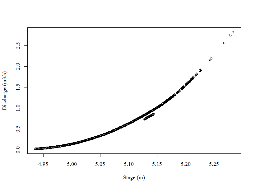
This code produced the following plot, which shows a clear exponential relationship between Stage and Discharge (with the exception of something strange going on between a stage of approximately 5.13 and 5.15 mm). I'm not sure what is going on here, and I have too many data points (17665 observations) to try to find these values.

I was wondering how I go about determining a regression equation that could be used to calculate the discharge (m3/s) based on the stage (m)? Thanks.

[startz]

lm(Discharge~exp(Stage, data = df)

[brant]

Thank you, is there a way to 1) plot this model over the original data to check how well it represents the data, and 2) determine the equation of the model? My datasheet has several values for "Stage" that do not have a corresponding discharge, and I want to be able to create a formula that I can use to calculate missing values for the discharge based on known values for stage.

[startz]

regressionResult <- lm(Discharge~exp(Stage, data = df)
summary(regressionResult)
prediction <- predict(regressionResult)

summary() will show you the coefficients for the equation and predict() will give you the predicted values. To predict from a different set of data, put it in a new dataframe like

newData <-data.frame(Stage = newStage)
predict(regressionResult, newData)

[brant]

Thank you. When I run the summary on the regressionResult, I receive the following output:

Call:
lm(formula = df$Discharge ~ exp(df$Stage))

Residuals:
     Min       1Q   Median       3Q      Max 
-0.07482 -0.05960 -0.01539  0.04806  1.22838 

Coefficients:
               Estimate Std. Error t value Pr(>|t|)    
(Intercept)   -4.117812   0.009718  -423.7   <2e-16 ***
exp(df$Stage)  0.028988   0.000065   446.0   <2e-16 ***
---
Signif. codes:  0 ‘***’ 0.001 ‘**’ 0.01 ‘*’ 0.05 ‘.’ 0.1 ‘ ’ 1

Residual standard error: 0.07444 on 17662 degrees of freedom
Multiple R-squared:  0.9184,	Adjusted R-squared:  0.9184 
F-statistic: 1.989e+05 on 1 and 17662 DF,  p-value: < 2.2e-16

How do I find the regression equation from this, and is there a way to plot the regression equation over my original data to check the fit of the model?

[startz]

The equation is Discharge = -4.1178 + 0.0289\times exp(Stage).
You can use lines() to add a line to a plot, using the values of your new data as the x variable and the values from predict() as the y variable.

[brant]

Sorry for my ignorance, but what is exp()? Is this the same as Discharge = -4.1178 + 0.0289^Stage? Or how would this be verified in excel?

[startz]

exp means exponential e^{0.289\times Stage}

[brant]

Is there a way to plot a trendline of this equation over my scatterplot to verify its accuracy?

[startz]

look at help for the lines() function

[brant]

Ok, I am clearly doing something wrong. When I ran the regression using the steps outlined by @startz, I got a discharge equation where Discharge = -4.1178 + 0.0289 x exp(Stage). The points on my curve follow a fairly clear regression pattern, which should mean that the regression equation should represent the data well. However, I ran a few of my first observations: Shown below:

Observation, Stage, Discharge
1, 5.042, 0.299
2, 5.043, 0.032
3, 5.044, 0.305
4, 5.045, 0.312
5, 5.044, 0.308

If I were to manually calculate each of the five Discharge values, based on the Stage, I would get:

1. Discharge = -4.1178 + 2.7182818 x exp(Stage) = -4.1178 + 2.7182181828459^ (0.28988 *5.042) = 0.19479
2. Discharge = -4.1178 + 2.7182818 x exp(Stage) =- 4.1178 + 2.7182181828459^ (0.28988 * 5.043) = 0.19605
3. Discharge = -4.1178 + 2.7182818 x exp(Stage) =-4.1178 + 2.7182181828459^ (0.28988 * 5.044) = 0.19729

As shown in the calculations above, the discharge formula that I created does not accurately calculate the discharge based on the stage of my data. Does anyone have any advice?

[startz]

Partially my fault. Should have been

e^{-4.1178+0.289\times Stage}

Note that the constant is part of the expression that goes into ```exp()``

[EconProf]

Consider the mtcars dataset. Suppose you want to estimate mpg as an exponential function of disp, or mpg = A*e^(B*disp). How can this nonlinear function be estimated using a linear regression model?

Because A = e^log(A), this equation can be rewritten as mpg = e^(log(A) + B*disp). Taking the natural log of both sides yields log(mgp) = log(A) + B*disp. This is linear with log(mpg) as the Y variable and disp as the X variable, log(A) as the intercept and B as the slope coefficient.

lm(log(mpg) ~ disp, mtcars) will estimate log(A) and B and thus estimate the coefficients for the nonlinear equation mgp = e^(log(A) + B*disp).

This is all due to the magical properties of the exponential function and its inverse, the natural log function.

lm(formula = log(mpg) ~ disp, data = mtcars)
#> 
#> Call:
#> lm(formula = log(mpg) ~ disp, data = mtcars)
#> 
#> Coefficients:
#> (Intercept)         disp  
#>    3.445548    -0.002115

# predicted mpg for a car with disp = 225, 
# which has actual mpg = 18.1

exp(3.445 - 0.002115*225)
#> [1] 19.47487

^{Created on 2024-01-14 with reprex v2.1.0}

[startz]

Everything @EconProf says is true (well duh!). But it's worth noting that a log equation and a nonlinear exponential equation are not the same because of the residuals. One is

y=A\times exp(b\times x) + \epsilon

The other is

log(y) = log(A) + b\times X+\epsilon

Note for the OP: You might actually want to have three coefficients:

y=C+A\times exp(b\times x) + \epsilon

[DaniMori]

How are you so sure the regression model follows an exponential equation? From what I see in the graph, it could well be a polynomial.

Also, you'd probably improve the fit if you could find some explanation for the few values slightly under the main ones around Stage = 5,13 m