Hello,
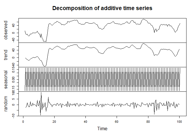
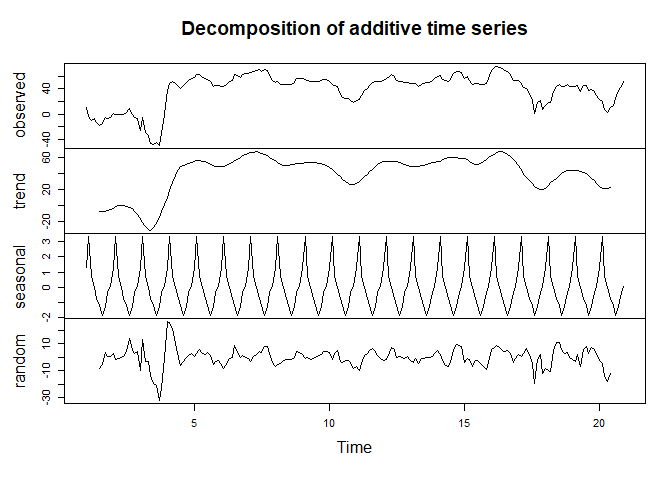
See below. I used the data you provided. I ran one run with frequency = 2 and another with frequency = 10. As you can see the decomposition changes given the "cycle". Hopefully this helps? You can explore the rest of the outputs by looking at output.
library(tidyverse)
df <- c(10.07, -4.08, -9.91, -7.41, -12.55, -17.25, -15.07, -4.93, -6.33, -4.93, 0.45, 0.12, -0.02, 0, -0.03, 1.97, 9.06, 0.07, -4.97, -6.98, -24.93, -4.87, -28.93, -33.57, -45.92, -48.29, -44.99, -48.93, -29.91, -0.01, 37.43, 48.06, 50.74, 47.57, 43.94, 40.97, 44.95, 49.64, 53.67, 56.01, 56.95, 62.08, 62.11, 57.99, 55.64, 55.13, 50.76, 42.91, 45.22, 45.63, 44, 43.88, 45.92, 51.07, 52.77, 62.89, 60.03, 58.19, 62.99, 63.52, 64.67, 65.24, 67.76, 68.41, 69.55, 67.28, 69.46, 68.38, 61.72, 53.72, 49.98, 50.73, 47.11, 47.07, 46.94, 47, 46.91, 49.59, 55.32, 55.78, 55.52, 55.23, 53.58, 51.74, 51.6, 51.41, 51.69, 52.59, 54.66, 54.1, 51.89, 46.58, 45.43, 43.96, 31.41, 26.9, 25.12, 24.12, 22.04, 18.37, 22.09, 23.35, 28.76, 36.63, 40.46, 45.85, 49.8, 51.36, 51.74, 51.92, 53.22, 56.62, 56.92, 61.64, 59.44, 52.75, 51.9, 51.38, 49.96, 50.29, 47.72, 48.38, 48.02, 44.23, 47.17, 48.19, 49.11, 50.44, 53.4, 56.55, 60.02, 60.22, 55, 52.39, 51.57, 54.71, 63.43, 67.37, 67.2, 66.03, 55.36, 58.59, 53.7, 46.03, 47.98, 47.84, 46.11, 46.08, 47.62, 55.77, 68.61, 74.15, 74.93, 73.59, 71.23, 68.79, 66.75, 62.47, 53.25, 53.26, 53.42, 47.91, 42.05, 40.96, 32.04, 20.82, 1.84, 17.94, 20.91, 7.78, 14.33, 18.56, 18.57, 35.81, 43.87, 46.93, 43.88, 43.85, 46.74, 43.94, 43.21, 43.81, 45.6, 35.21, 45.64, 45.63, 37.94, 39.53, 35.97, 29.72, 22.55, 20.04, 7.24, 3.43, 10.04, 14.2, 25.41, 36.98, 43.89, 50.98) %>% as.data.frame()
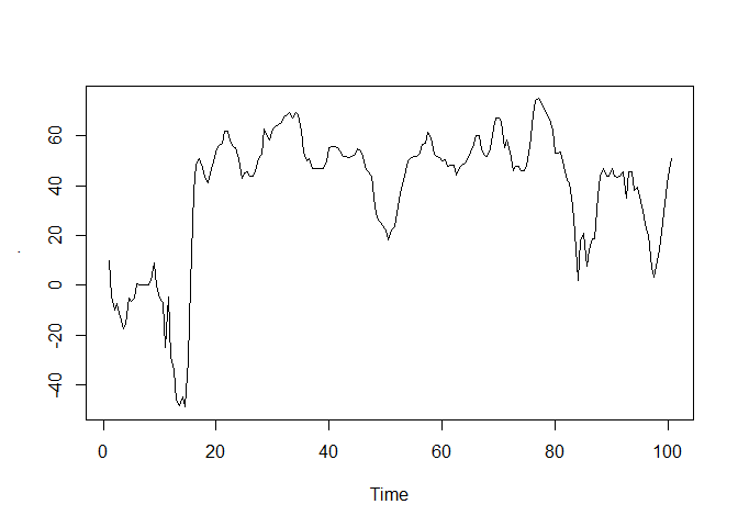
TS <- ts(df, frequency = 2)
output <- decompose(TS)
plot.ts(TS)
plot(output)
library(tidyverse)
df <- c(10.07, -4.08, -9.91, -7.41, -12.55, -17.25, -15.07, -4.93, -6.33, -4.93, 0.45, 0.12, -0.02, 0, -0.03, 1.97, 9.06, 0.07, -4.97, -6.98, -24.93, -4.87, -28.93, -33.57, -45.92, -48.29, -44.99, -48.93, -29.91, -0.01, 37.43, 48.06, 50.74, 47.57, 43.94, 40.97, 44.95, 49.64, 53.67, 56.01, 56.95, 62.08, 62.11, 57.99, 55.64, 55.13, 50.76, 42.91, 45.22, 45.63, 44, 43.88, 45.92, 51.07, 52.77, 62.89, 60.03, 58.19, 62.99, 63.52, 64.67, 65.24, 67.76, 68.41, 69.55, 67.28, 69.46, 68.38, 61.72, 53.72, 49.98, 50.73, 47.11, 47.07, 46.94, 47, 46.91, 49.59, 55.32, 55.78, 55.52, 55.23, 53.58, 51.74, 51.6, 51.41, 51.69, 52.59, 54.66, 54.1, 51.89, 46.58, 45.43, 43.96, 31.41, 26.9, 25.12, 24.12, 22.04, 18.37, 22.09, 23.35, 28.76, 36.63, 40.46, 45.85, 49.8, 51.36, 51.74, 51.92, 53.22, 56.62, 56.92, 61.64, 59.44, 52.75, 51.9, 51.38, 49.96, 50.29, 47.72, 48.38, 48.02, 44.23, 47.17, 48.19, 49.11, 50.44, 53.4, 56.55, 60.02, 60.22, 55, 52.39, 51.57, 54.71, 63.43, 67.37, 67.2, 66.03, 55.36, 58.59, 53.7, 46.03, 47.98, 47.84, 46.11, 46.08, 47.62, 55.77, 68.61, 74.15, 74.93, 73.59, 71.23, 68.79, 66.75, 62.47, 53.25, 53.26, 53.42, 47.91, 42.05, 40.96, 32.04, 20.82, 1.84, 17.94, 20.91, 7.78, 14.33, 18.56, 18.57, 35.81, 43.87, 46.93, 43.88, 43.85, 46.74, 43.94, 43.21, 43.81, 45.6, 35.21, 45.64, 45.63, 37.94, 39.53, 35.97, 29.72, 22.55, 20.04, 7.24, 3.43, 10.04, 14.2, 25.41, 36.98, 43.89, 50.98)
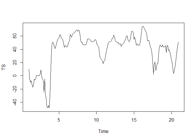
TS <- ts(df, frequency = 10)
output <- decompose(TS)
plot.ts(TS)
plot(output)
Created on 2020-10-29 by the reprex package (v0.3.0)
 see how to do a reprex and then I can have a look tonight.