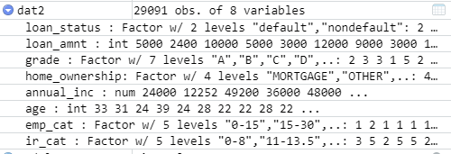
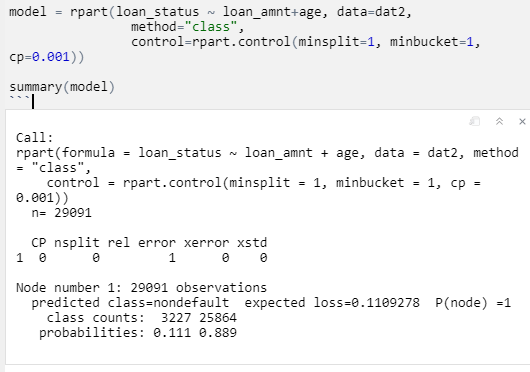
You are not getting any splitting. I have never used fancyRpartPlot but it seems it does not like model with no splits. Here is an example using a built-in data set showing what the summary should look like.
library(rpart)
#> Warning: package 'rpart' was built under R version 3.5.3
fit <- rpart(Kyphosis ~ Age + Number + Start, data = kyphosis, method = "class")

summary(fit)
#> Call:
#> rpart(formula = Kyphosis ~ Age + Number + Start, data = kyphosis,
#>     method = "class")
#>   n= 81
#>
#>           CP nsplit rel error   xerror      xstd
#> 1 0.17647059      0 1.0000000 1.000000 0.2155872
#> 2 0.01960784      1 0.8235294 1.058824 0.2200975
#> 3 0.01000000      4 0.7647059 1.058824 0.2200975
#>
#> Variable importance
#>  Start    Age Number
#>     64     24     12
#>
#> Node number 1: 81 observations,    complexity param=0.1764706
#>   predicted class=absent   expected loss=0.2098765  P(node) =1
#>     class counts:    64    17
#>    probabilities: 0.790 0.210
#>   left son=2 (62 obs) right son=3 (19 obs)
#>   Primary splits:
#>       Start  < 8.5  to the right, improve=6.762330, (0 missing)
#>       Number < 5.5  to the left,  improve=2.866795, (0 missing)
#>       Age    < 39.5 to the left,  improve=2.250212, (0 missing)
#>   Surrogate splits:
#>       Number < 6.5  to the left,  agree=0.802, adj=0.158, (0 split)
#>
#> Node number 2: 62 observations,    complexity param=0.01960784
#>   predicted class=absent   expected loss=0.09677419  P(node) =0.7654321
#>     class counts:    56     6
#>    probabilities: 0.903 0.097
#>   left son=4 (29 obs) right son=5 (33 obs)
#>   Primary splits:
#>       Start  < 14.5 to the right, improve=1.0205280, (0 missing)
#>       Age    < 55   to the left,  improve=0.6848635, (0 missing)
#>       Number < 4.5  to the left,  improve=0.2975332, (0 missing)
#>   Surrogate splits:
#>       Number < 3.5  to the left,  agree=0.645, adj=0.241, (0 split)
#>       Age    < 16   to the left,  agree=0.597, adj=0.138, (0 split)
#>
#> Node number 3: 19 observations
#>   predicted class=present  expected loss=0.4210526  P(node) =0.2345679
#>     class counts:     8    11
#>    probabilities: 0.421 0.579
#>
#> Node number 4: 29 observations
#>   predicted class=absent   expected loss=0  P(node) =0.3580247
#>     class counts:    29     0
#>    probabilities: 1.000 0.000
#>
#> Node number 5: 33 observations,    complexity param=0.01960784
#>   predicted class=absent   expected loss=0.1818182  P(node) =0.4074074
#>     class counts:    27     6
#>    probabilities: 0.818 0.182
#>   left son=10 (12 obs) right son=11 (21 obs)
#>   Primary splits:
#>       Age    < 55   to the left,  improve=1.2467530, (0 missing)
#>       Start  < 12.5 to the right, improve=0.2887701, (0 missing)
#>       Number < 3.5  to the right, improve=0.1753247, (0 missing)
#>   Surrogate splits:
#>       Start  < 9.5  to the left,  agree=0.758, adj=0.333, (0 split)
#>       Number < 5.5  to the right, agree=0.697, adj=0.167, (0 split)
#>
#> Node number 10: 12 observations
#>   predicted class=absent   expected loss=0  P(node) =0.1481481
#>     class counts:    12     0
#>    probabilities: 1.000 0.000
#>
#> Node number 11: 21 observations,    complexity param=0.01960784
#>   predicted class=absent   expected loss=0.2857143  P(node) =0.2592593
#>     class counts:    15     6
#>    probabilities: 0.714 0.286
#>   left son=22 (14 obs) right son=23 (7 obs)
#>   Primary splits:
#>       Age    < 111  to the right, improve=1.71428600, (0 missing)
#>       Start  < 12.5 to the right, improve=0.79365080, (0 missing)
#>       Number < 3.5  to the right, improve=0.07142857, (0 missing)
#>
#> Node number 22: 14 observations
#>   predicted class=absent   expected loss=0.1428571  P(node) =0.1728395
#>     class counts:    12     2
#>    probabilities: 0.857 0.143
#>
#> Node number 23: 7 observations
#>   predicted class=present  expected loss=0.4285714  P(node) =0.08641975
#>     class counts:     3     4
#>    probabilities: 0.429 0.571
Created on 2019-11-04 by the reprex package (v0.3.0.9000)

