Data Labeling Stacked Bar Chart

vafowler · August 28, 2023, 3:29pm

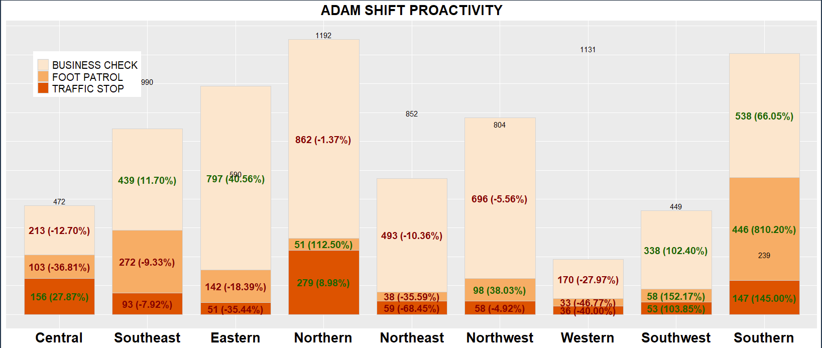
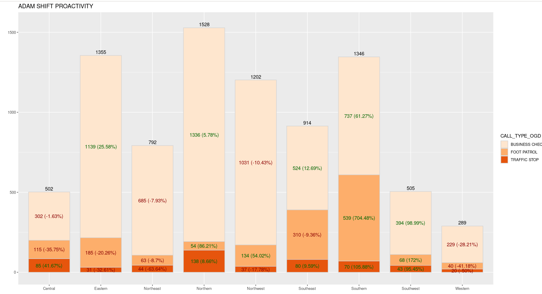
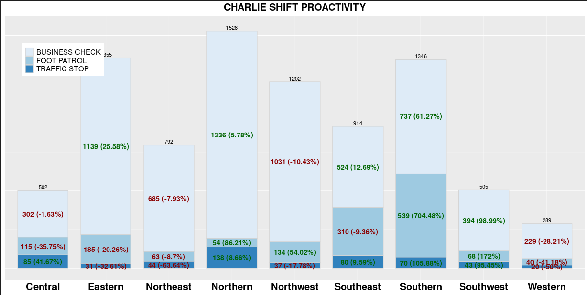
I am attempting to add Column total call out above each column. Here is how my data frame is set up. I will also mention that I am unable to share the complete data but will provide as much as possible. Columns NEW_DIST , CALL_TYPE_OGD (has 3 different chr values), SHIFT (A), Pct_Change, STATUS (Current), COUNT, DIST_COUNT. I currently have the CALL_TYPE_OGD Count and Pct_Change labeled. I want to add the DIST_COUNT above each stacked column. The DIST_COUNT number does not need to be summed. I only need to use one value per NEW_DIST. Not sure if I am making sense.

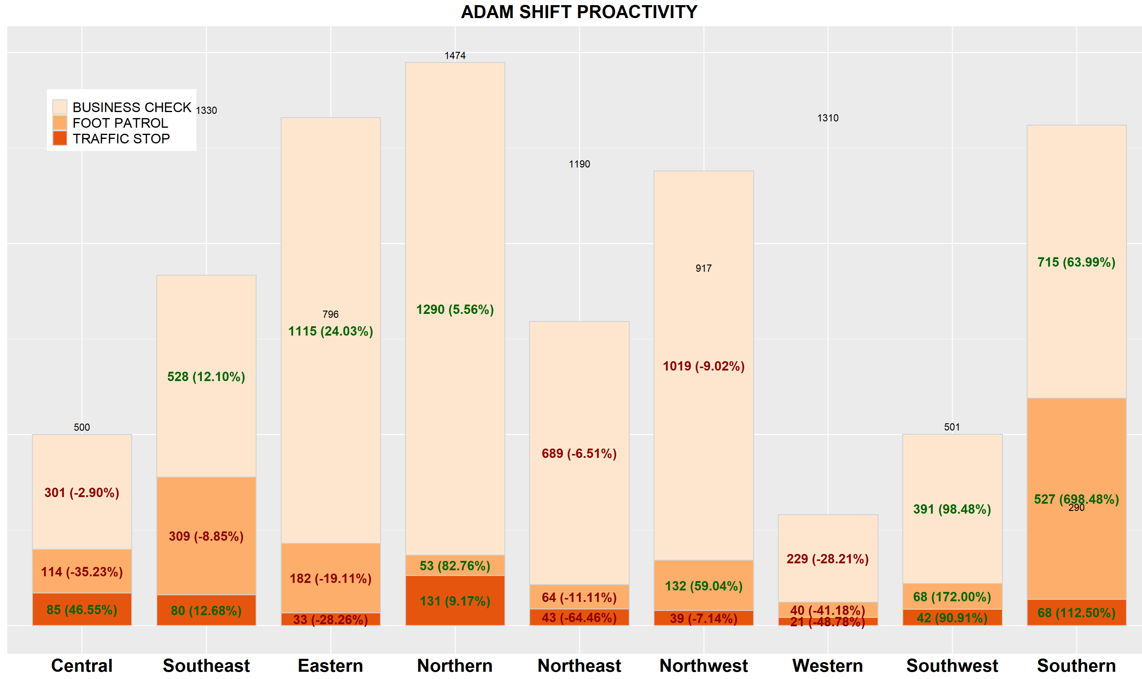
plot <- ggplot(fd1, aes(x = NEW_DIST, y = COUNT, fill = CALL_TYPE_OGD)) +
  geom_bar(position = "stack", stat = "identity", width = 0.8, color = "light gray") +
  labs(
    title = "ADAM SHIFT PROACTIVITY",
    x = "",
    y = "",
    fill = "CALL_TYPE_OGD"
  ) +
  scale_fill_brewer(type = "seq", palette = 'Oranges') +
  # Add data labels using geom_text
  geom_text(
    aes(label = paste0(COUNT, " (", Pct_Change, "%)")),  # Include both raw count and percentage change
    position = position_stack(vjust = 0.5),  
    color = ifelse(fd$Pct_Change >= 0, "darkgreen", "darkred"),  
    hjust = ifelse(fd$Pct_Change >= 0.5, 0.5, 0.5),  
    size = 4)

print(plot)

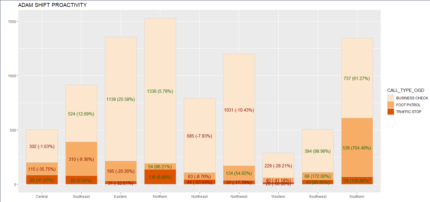
The plot is produced with the code provided above.

Please let me know if I need to provide further clarification or more of the script. I attempted to upload the data frame that was usable but couldn't figure out. Below is the df
"NEW_DIST" "CALL_TYPE_OGD" "SHIFT" "Pct_Change" "STATUS" "COUNT" "DIST_COUNT"
"Central" "BUSINESS CHECK" "A" "-1.63" "CURRENT" 302 502
"Central" "FOOT PATROL" "A" "-35.75" "CURRENT" 115 502
"Central" "TRAFFIC STOP" "A" "41.67" "CURRENT" 85 502
"Eastern" "BUSINESS CHECK" "A" "25.58" "CURRENT" 1139 1355
"Eastern" "FOOT PATROL" "A" "-20.26" "CURRENT" 185 1355
"Eastern" "TRAFFIC STOP" "A" "-32.61" "CURRENT" 31 1355
"Northeast" "BUSINESS CHECK" "A" "-7.93" "CURRENT" 685 792
"Northeast" "FOOT PATROL" "A" "-8.70" "CURRENT" 63 792
"Northeast" "TRAFFIC STOP" "A" "-63.64" "CURRENT" 44 792
"Northern" "BUSINESS CHECK""A" "5.78" "CURRENT" 1336 1528
"Northern" "FOOT PATROL" "A" "86.21" "CURRENT" 54 1528
"Northern" "TRAFFIC STOP" "A" "8.66" "CURRENT" 138 1528
"Northwest" "BUSINESS CHECK""A" "-10.43" "CURRENT" 1031 1202
"Northwest" "FOOT PATROL" "A" "54.02" "CURRENT" 134 1202
"Northwest" "TRAFFIC STOP" "A" "-17.78" "CURRENT" 37 1202
"Southeast" "BUSINESS CHECK""A" "12.69" "CURRENT" 524 914
"Southeast" "FOOT PATROL" "A" "-9.36" "CURRENT" 310 914
"Southeast" "TRAFFIC STOP" "A" "9.59" CURRENT" 80 914
"Southern" "BUSINESS CHECK""A" "61.27" "CURRENT" 737 1346
"Southern" "FOOT PATROL" "A" "704.48" "CURRENT" 539 1346
"Southern" "TRAFFIC STOP" "A" "105.88" "CURRENT" 70 1346
"Southwest" "BUSINESS CHECK""A" "98.99" "CURRENT" 394 505
"Southwest" "FOOT PATROL" "A" "172.00" "CURRENT" 68 505
"Southwest" "TRAFFIC STOP" "A" "95.45" "CURRENT" 43 505
"Western" "BUSINESS CHECK""A" "-28.21" "CURRENT" 229 289
"Western" "FOOT PATROL" "A" "-41.18" "CURRENT" 40 289
"Western" "TRAFFIC STOP" "A" "-50.00" "CURRENT" 20 289

jrkrideau · August 28, 2023, 4:44pm

Hi, welcome to the forum

That sample dataset has some quote and spacing problems.

For example

"Northern" "BUSINESS CHECK""A" "5.78" "CURRENT" 1336 1528

A handy way to supply some sample data is the dput() function. In the case of a large dataset something like dput(head(mydata, 100)) should supply the data we need. Just do dput(mydata) where mydata is your data. Copy the output and paste it here.

As a new member of the forum you may find FAQ Asking Questions to be useful.

I think I've got the data cleaned up. Here it is in dput() format

structure(list(NEW_DIST = c("Central", "Central", "Central", 
"Eastern", "Eastern", "Eastern", "Northeast", "Northeast", "Northeast", 
"Northern", "Northern", "Northern", "Northwest", "Northwest", 
"Northwest", "Southeast", "Southeast", "Southeast", "Southern", 
"Southern", "Southern", "Southwest", "Southwest", "Southwest", 
"Western", "Western", "Western"), CALL_TYPE_OGD = c("BUSINESS CHECK", 
"FOOT PATROL", "TRAFFIC STOP", "BUSINESS CHECK", "FOOT PATROL", 
"TRAFFIC STOP", "BUSINESS CHECK", "FOOT PATROL", "TRAFFIC STOP", 
"BUSINESS CHECK", "FOOT PATROL", "TRAFFIC STOP", "BUSINESS CHECK", 
"FOOT PATROL", "TRAFFIC STOP", "BUSINESS CHECK", "FOOT PATROL", 
"TRAFFIC STOP", "BUSINESS CHECK", "FOOT PATROL", "TRAFFIC STOP", 
"BUSINESS CHECK", "FOOT PATROL", "TRAFFIC STOP", "BUSINESS CHECK", 
"FOOT PATROL", "TRAFFIC STOP"), SHIFT = c("A", "A", "A", "A", 
"A", "A", "A", "A", "A", "A", "A", "A", "A", "A", "A", "A", "A", 
"A", "A", "A", "A", "A", "A", "A", "A", "A", "A"), Pct_Change = c(-1.63, 
-35.75, 41.67, 25.58, -20.26, -32.61, -7.93, -8.7, -63.64, 5.78, 
86.21, 8.66, -10.43, 54.02, -17.78, 12.69, -9.36, 9.59, 61.27, 
704.48, 105.88, 98.99, 172, 95.45, -28.21, -41.18, -50), STATUS = c("CURRENT", 
"CURRENT", "CURRENT", "CURRENT", "CURRENT", "CURRENT", "CURRENT", 
"CURRENT", "CURRENT", "CURRENT", "CURRENT", "CURRENT", "CURRENT", 
"CURRENT", "CURRENT", "CURRENT", "CURRENT", "CURRENT", "CURRENT", 
"CURRENT", "CURRENT", "CURRENT", "CURRENT", "CURRENT", "CURRENT", 
"CURRENT", "CURRENT"), COUNT = c(302L, 115L, 85L, 1139L, 185L, 
31L, 685L, 63L, 44L, 1336L, 54L, 138L, 1031L, 134L, 37L, 524L, 
310L, 80L, 737L, 539L, 70L, 394L, 68L, 43L, 229L, 40L, 20L), 
    DIST_COUNT = c(502L, 502L, 502L, 1355L, 1355L, 1355L, 792L, 
    792L, 792L, 1528L, 1528L, 1528L, 1202L, 1202L, 1202L, 914L, 
    914L, 914L, 1346L, 1346L, 1346L, 505L, 505L, 505L, 289L, 
    289L, 289L)), row.names = c(NA, -27L), class = "data.frame")

vafowler · August 28, 2023, 5:56pm

I appreciate the quick tutorial, and will use it in the future. Any help regarding my labeling issue?

jrkrideau · August 28, 2023, 6:02pm

Are you asking how to place the numbers on the plot or how to extract the numbers from the data set?

vafowler · August 28, 2023, 6:14pm

I am asking how to keep the bar plot I posted how it is but add the column total at the top of each column. The column total is the DIST_COUNT. I only need 1 total per column versus summing all the DIST_COUNT for each column

jrkrideau · August 28, 2023, 7:00pm

Okay I think I've got it but I am going to be using {data.table} to get the numbers

Assuming your data is called fd1

library(ggplot2
library(data.table)

fd1 <- as.data.table(fd1)

## grab first entry in data grouped by NEW_DIST
tp_num  <- fd1[, .SD[1], .SDcols = "DIST_COUNT", by = NEW_DIST]

## Get vector of numbers
nums  <- tp_num[, DIST_COUNT]


p1  <- ggplot(fd1, aes(x = NEW_DIST, y = COUNT, fill = CALL_TYPE_OGD)) +
  geom_bar(position = "stack", stat = "identity", width = 0.8, color = "light gray") +
  labs(
    title = "ADAM SHIFT PROACTIVITY",
    x = "",
    y = "",
    fill = "CALL_TYPE_OGD"
  ) +
  scale_fill_brewer(type = "seq", palette = 'Oranges') +
  # Add data labels using geom_text
  geom_text(
    aes(label = paste0(COUNT, " (", Pct_Change, "%)")),  # Include both raw count and percentage change
    position = position_stack(vjust = 0.5),  
    color = ifelse(fd1$Pct_Change >= 0, "darkgreen", "darkred"),  
    hjust = ifelse(fd1$Pct_Change >= 0.5, 0.5, 0.5),  
    size = 4) +
  annotate("text", x = 1:9, y = nums + 20, label = as.character(nums))

vafowler · August 29, 2023, 12:17pm

This is great! Thank you so much for your help! I added the above to my current script.
Is there a way to adjust/ standardize the position above the column?

Also, This fix doesn't work for my other shifts. The plot doesn't populate. I have the same issue with my Charlie Shift. Charlie Shift uses the same code as below but with c instead of b in the names.
UPDATE: I was able to get it to work on my other shifts

fdb1 <- fdb %>%
  group_by(NEW_DIST) %>%
  mutate(DIST_COUNT = sum(COUNT)) %>%
  ungroup()

fdb1 <- as.data.table(fdb1)

## grab first entry in data grouped by NEW_DIST
tp_num  <- fdb1[, .SD[1], .SDcols = "DIST_COUNT", by = NEW_DIST]

## Get vector of numbers
nums  <- tp_num[, DIST_COUNT]

plotb <- ggplot(fdb1, aes(x = NEW_DIST, y = COUNT, fill = CALL_TYPE_OGD)) +
  geom_bar(position = "stack", stat = "identity", width = 0.8, color = "light gray") +
  labs(
    title = "BAKER SHIFT PROACTIVITY",
    x = "",
    y = "",
    fill = "CALL_TYPE_OGD"
  ) +
  scale_fill_brewer(type = "seq", palette = 'Purples') +
  # Add data labels using geom_text
  geom_text(
    aes(label = paste0(COUNT, " (", Pct_Change, "%)")),  # Include both raw count and percentage change
    position = position_stack(vjust = 0.5),  
    color = ifelse(fdb1$Pct_Change >= 0, "darkgreen", "darkred"),  
    hjust = ifelse(fdb1$Pct_Change >= 0.5, 0.5, 0.5),  
    size = 5,
    fontface = "bold") +
  theme(plot.title = element_text(face = "bold", size = 20,hjust = 0.5),
      axis.ticks.x=element_blank(),
      axis.text.x=element_text(size = 20, color = "black", face = "bold"), #x axis label#
      axis.text.y=element_blank(),
      axis.ticks.y=element_blank(),
      axis.title.x=element_blank(),
      axis.title.y=element_blank(),
      strip.text.x = element_text(size = 16, color = "black", face = "bold"), #legend font##
      legend.text = element_text(size = 15),
      legend.position = c(.1,0.9),
      legend.justification = c("top"),
      legend.title = element_blank()) +
   annotate("text", x = 1:9, y = nums + 20, label = as.character(nums))
 
print(plotb)

jrkrideau · August 29, 2023, 1:03pm

Quick response re the plot. I think your script is very subtly different from mine as I get

You may have to supply us with a new copy of your code.

I save this plot using

png("vfowler2.png", width = 1000, height = 480)
p1
dev.off()

as I was having a problem getting the height-width ratios right in ggplot2.

I should be able to get to the code in an hour or two. Can you give us a sample of the Charlie Shift data using dput()

vafowler · August 29, 2023, 1:12pm

Sample of Charlie Shift Data

dput(fdc1)
structure(list(NEW_DIST = structure(c(1L, 1L, 1L, 3L, 3L, 3L, 
3L, 5L, 5L, 5L, 4L, 4L, 4L, 4L, 6L, 6L, 6L, 6L, 2L, 2L, 2L, 2L, 
9L, 9L, 9L, 8L, 8L, 8L, 7L, 7L, 7L, 1L, 5L, 9L), levels = c("Central", 
"Southeast", "Eastern", "Northern", "Northeast", "Northwest", 
"Western", "Southwest", "Southern"), class = "factor"), CALL_TYPE_OGD = c("BUSINESS CHECK", 
"FOOT PATROL", "TRAFFIC STOP", "BIKE PATROL", "BUSINESS CHECK", 
"FOOT PATROL", "TRAFFIC STOP", "BUSINESS CHECK", "FOOT PATROL", 
"TRAFFIC STOP", "BIKE PATROL", "BUSINESS CHECK", "FOOT PATROL", 
"TRAFFIC STOP", "BIKE PATROL", "BUSINESS CHECK", "FOOT PATROL", 
"TRAFFIC STOP", "BIKE PATROL", "BUSINESS CHECK", "FOOT PATROL", 
"TRAFFIC STOP", "BUSINESS CHECK", "FOOT PATROL", "TRAFFIC STOP", 
"BUSINESS CHECK", "FOOT PATROL", "TRAFFIC STOP", "BUSINESS CHECK", 
"FOOT PATROL", "TRAFFIC STOP", "BIKE PATROL", "BIKE PATROL", 
"BIKE PATROL"), Pct_Change = c("-21.91", "-45.59", "8.14", "-69.44", 
"3.09", "-14.29", "-23.73", "-16.85", "-32.73", "-11.70", "20.69", 
"-2.46", "-18.84", "-38.64", "200.00", "-20.63", "-14.77", "-19.52", 
"-75.00", "1.80", "-5.38", "6.25", "28.05", "183.26", "-3.20", 
"-9.04", "148.33", "26.25", "-27.60", "-31.43", "-14.48", "-100.00", 
"-100.00", "-100.00"), STATUS = c("CURRENT", "CURRENT", "CURRENT", 
"CURRENT", "CURRENT", "CURRENT", "CURRENT", "CURRENT", "CURRENT", 
"CURRENT", "CURRENT", "CURRENT", "CURRENT", "CURRENT", "CURRENT", 
"CURRENT", "CURRENT", "CURRENT", "CURRENT", "CURRENT", "CURRENT", 
"CURRENT", "CURRENT", "CURRENT", "CURRENT", "CURRENT", "CURRENT", 
"CURRENT", "CURRENT", "CURRENT", "CURRENT", "CURRENT", "CURRENT", 
"CURRENT"), COUNT = c(253, 142, 93, 22, 701, 540, 225, 296, 187, 
385, 70, 834, 224, 162, 3, 735, 329, 202, 1, 452, 246, 170, 566, 
609, 333, 322, 149, 101, 202, 144, 124, 0, 0, 0), DIST_COUNT = c(488, 
488, 488, 1488, 1488, 1488, 1488, 868, 868, 868, 1290, 1290, 
1290, 1290, 1269, 1269, 1269, 1269, 869, 869, 869, 869, 1508, 
1508, 1508, 572, 572, 572, 470, 470, 470, 488, 868, 1508)), row.names = c(NA, 
-34L), class = c("data.table", "data.frame"), .internal.selfref = <pointer: 0x000001ebbed85930>)

Below is the exact code I ran to obtain the plot at the bottom.

fdc1 <- fdc %>%
  group_by(NEW_DIST) %>%
  mutate(DIST_COUNT = sum(COUNT)) %>%
  ungroup()

fdc1 <- as.data.table(fdc1)

## grab first entry in data grouped by NEW_DIST
tp_num  <- fdc1[, .SD[1], .SDcols = "DIST_COUNT", by = NEW_DIST]

## Get vector of numbers
nums  <- tp_num[, DIST_COUNT]


plotc <- ggplot(fdc1, aes(x = NEW_DIST, y = COUNT, fill = CALL_TYPE_OGD)) +
  geom_bar(position = "stack", stat = "identity", width = 0.8, color = "light gray") +
  labs(
    title = "CHARLIE SHIFT PROACTIVITY",
    x = "",
    y = "",
    fill = "CALL_TYPE_OGD"
  ) +
  scale_fill_brewer(type = "seq", palette = 'Blues') +
  # Add data labels using geom_text
  geom_text(
    aes(label = paste0(COUNT, " (", Pct_Change, "%)")),  # Include both raw count and percentage change
    position = position_stack(vjust = 0.5),  
    color = ifelse(fdc1$Pct_Change >= 0, "darkgreen", "darkred"),  
    hjust = ifelse(fdc1$Pct_Change >= 0.5, 0.5, 0.5),  
    size = 5,
    fontface = "bold") +
  theme(plot.title = element_text(face = "bold", size = 20,hjust = 0.5),
    axis.ticks.x=element_blank(),
    axis.text.x=element_text(size = 20, color = "black", face = "bold"), #x axis label#
    axis.text.y=element_blank(),
    axis.ticks.y=element_blank(),
    axis.title.x=element_blank(),
    axis.title.y=element_blank(),
    strip.text.x = element_text(size = 16, color = "black", face = "bold"), #legend font##
    legend.text = element_text(size = 15),
    legend.position = c(.1,0.9),
    legend.justification = c("top"),
    legend.title = element_blank()) +
  annotate("text", x = 1:9, y = nums + 20, label = as.character(nums))
  
print(plotc)

jrkrideau · August 29, 2023, 4:16pm

I ran your code using the Adam Shift data and got essentially the same thing as before.

The only differences that I see are that I loaded the .csv file as a data.table.

fd1  <- fread("data/cop1.csv")  ## Your original data set.

and rather than use

fdc1 <- fdc %>%
  group_by(NEW_DIST) %>%
  mutate(DIST_COUNT = sum(COUNT)) %>%
  ungroup()

I did

fd1[, DIST_COUNT := sum(COUNT),  by = "NEW_DIST" ]
fdc1 <- fd1

and I have a problem seeing why this should make a significant difference.

RStudio is refusing to upload the plot, probably due to heavy use. You should be able to download it frob vfowler3

Could you supply the output of

Thanks

vafowler · August 30, 2023, 4:53pm

Below is the output of the vfowler3

I reran the script using the changes you mentioned. My final plot is still showing the numbers all over the place
Here is the script. The data can be found after the script.

fd1 <- as.data.table(fd)
fd1[, DIST_COUNT := sum(COUNT),  by = "NEW_DIST" ]
fd1 <- na.omit(fd1)
tp_num  <- fd1[, .SD[1], .SDcols = "DIST_COUNT", by = NEW_DIST]

## Get vector of numbers
nums  <- tp_num[, DIST_COUNT]

plota <- ggplot(fd1, aes(x = NEW_DIST, y = COUNT, fill = CALL_TYPE_OGD)) +
  geom_bar(position = "stack", stat = "identity", width = 0.8, color = "light gray") +
  labs(
    title = "ADAM SHIFT PROACTIVITY",
    x = "",
    y = "",
    fill = "CALL_TYPE_OGD"
  ) +
  scale_fill_brewer(type = "seq", palette = 'Oranges') +
  # Add data labels using geom_text
  geom_text(
    aes(label = paste0(COUNT, " (", Pct_Change, "%)")),  # Include both raw count and percentage change
    position = position_stack(vjust = 0.5),  
    color = ifelse(fd1$Pct_Change >= 0, "darkgreen", "darkred"),  
    hjust = ifelse(fd1$Pct_Change >= 0.5, 0.5, 0.5),  
    size = 5,
    fontface = "bold") +
  theme(plot.title = element_text(face = "bold", size = 20,hjust = 0.5),
        axis.ticks.x=element_blank(),
        axis.text.x=element_text(size = 20, color = "black", face = "bold"), #x axis label#
        axis.text.y=element_blank(),
        axis.ticks.y=element_blank(),
        axis.title.x=element_blank(),
        axis.title.y=element_blank(),
        strip.text.x = element_text(size = 16, color = "black", face = "bold"), #legend font##
        legend.text = element_text(size = 15),
        legend.position = c(.1,0.9),
        legend.justification = c("top"),
        legend.title = element_blank()) +
  annotate("text", x = 1:9, y = nums + 20, label = as.character(nums))

print(plota)

dput(fd1)
structure(list(NEW_DIST = structure(c(1L, 1L, 1L, 3L, 3L, 3L, 
5L, 5L, 5L, 4L, 4L, 4L, 6L, 6L, 6L, 2L, 2L, 2L, 9L, 9L, 9L, 8L, 
8L, 8L, 7L, 7L, 7L), levels = c("Central", "Southeast", "Eastern", 
"Northern", "Northeast", "Northwest", "Western", "Southwest", 
"Southern"), class = "factor"), CALL_TYPE_OGD = c("BUSINESS CHECK", 
"FOOT PATROL", "TRAFFIC STOP", "BUSINESS CHECK", "FOOT PATROL", 
"TRAFFIC STOP", "BUSINESS CHECK", "FOOT PATROL", "TRAFFIC STOP", 
"BUSINESS CHECK", "FOOT PATROL", "TRAFFIC STOP", "BUSINESS CHECK", 
"FOOT PATROL", "TRAFFIC STOP", "BUSINESS CHECK", "FOOT PATROL", 
"TRAFFIC STOP", "BUSINESS CHECK", "FOOT PATROL", "TRAFFIC STOP", 
"BUSINESS CHECK", "FOOT PATROL", "TRAFFIC STOP", "BUSINESS CHECK", 
"FOOT PATROL", "TRAFFIC STOP"), SHIFT = c("A", "A", "A", "A", 
"A", "A", "A", "A", "A", "A", "A", "A", "A", "A", "A", "A", "A", 
"A", "A", "A", "A", "A", "A", "A", "A", "A", "A"), Pct_Change = c("-2.90", 
"-35.23", "46.55", "24.03", "-19.11", "-28.26", "-6.51", "-11.11", 
"-64.46", "5.56", "82.76", "9.17", "-9.02", "59.04", "-7.14", 
"12.10", "-8.85", "12.68", "63.99", "698.48", "112.50", "98.48", 
"172.00", "90.91", "-28.21", "-41.18", "-48.78"), STATUS = c("CURRENT", 
"CURRENT", "CURRENT", "CURRENT", "CURRENT", "CURRENT", "CURRENT", 
"CURRENT", "CURRENT", "CURRENT", "CURRENT", "CURRENT", "CURRENT", 
"CURRENT", "CURRENT", "CURRENT", "CURRENT", "CURRENT", "CURRENT", 
"CURRENT", "CURRENT", "CURRENT", "CURRENT", "CURRENT", "CURRENT", 
"CURRENT", "CURRENT"), COUNT = c(301L, 114L, 85L, 1115L, 182L, 
33L, 689L, 64L, 43L, 1290L, 53L, 131L, 1019L, 132L, 39L, 528L, 
309L, 80L, 715L, 527L, 68L, 391L, 68L, 42L, 229L, 40L, 21L), 
   DIST_COUNT = c(500L, 500L, 500L, 1330L, 1330L, 1330L, 796L, 
   796L, 796L, 1474L, 1474L, 1474L, 1190L, 1190L, 1190L, 917L, 
   917L, 917L, 1310L, 1310L, 1310L, 501L, 501L, 501L, 290L, 
   290L, 290L)), row.names = c(NA, -27L), groups = structure(list(
   NEW_DIST = structure(c(1L, 2L, 3L, 4L, 5L, 6L, 7L, 8L, 9L, 
   NA), levels = c("Central", "Southeast", "Eastern", "Northern", 
   "Northeast", "Northwest", "Western", "Southwest", "Southern"
   ), class = "factor"), .rows = structure(list(1:3, 16:18, 
       4:6, 10:12, 7:9, 13:15, 28:30, 22:24, 19:21, 25:27), ptype = integer(0), class = c("vctrs_list_of", 
   "vctrs_vctr", "list"))), row.names = c(NA, -10L), .drop = TRUE, class = c("tbl_df", 
"tbl", "data.frame")), class = c("data.table", "data.frame"), .internal.selfref = <pointer: 0x0000012833954b80>)

vafowler · August 31, 2023, 12:29pm

I figured out why my numbers do not align with the columns are yours do. I have my NEW_DIST in a specific order and yours is in alphabetical order. Thank you so much for all of your help.

jrkrideau · August 31, 2023, 7:32pm

Argh!!
I saw that in the dput() and failed to recognize the problem. Sorry, my stupidity.

system · October 12, 2023, 7:33pm

This topic was automatically closed 42 days after the last reply. New replies are no longer allowed.

If you have a query related to it or one of the replies, start a new topic and refer back with a link.