Dashed Line in ggplot does not show up in the right style in the legend

[JonasM]

Hi All

I work with ggplot and I have a problem with the legend.
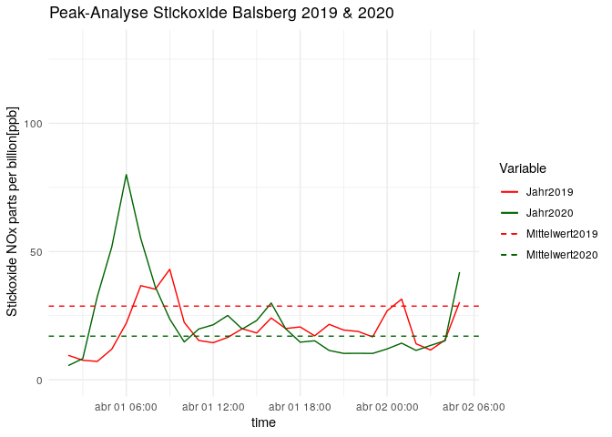
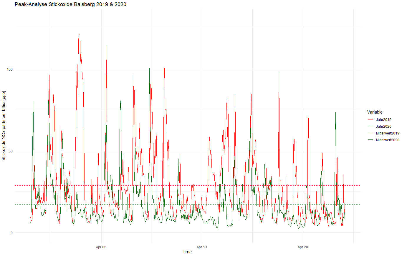
The dashed lines in the plot are not dashed in the legend, even though I defined their style with the command: scale_linetype_manual
Suspicious is also, I do not receive a warning or error in the console. However, it is not executed.
Here is my code, followed by the plot:

ggplot(nox, aes(x=Zeit))+
  geom_line(aes(y=Jahr2019,color="Jahr2019"))+
  geom_line(aes(y=Jahr2020,color="Jahr2020"))+
  geom_hline(aes(color="Mittelwert2019",yintercept=28.72),linetype="dashed",size=0.5)+
  geom_hline(aes(color="Mittelwert2020",yintercept=17.01),linetype="dashed",size=0.5)+
  ylim(0,130)+
  ggtitle("Peak-Analyse Stickoxide Balsberg 2019 & 2020")+
  labs(x="time",
       y=" Stickoxide NOx parts per billion[ppb]")+
  scale_color_manual(name="Variable",
                     breaks = c("Jahr2019", "Jahr2020", "Mittelwert2019", "Mittelwert2020"),
                     values = c("Jahr2019" = "red", "Jahr2020" = "darkgreen", "Mittelwert2019"="Red","Mittelwert2020"="Darkgreen"))+
  scale_linetype_manual(breaks = c("Jahr2019", "Jahr2020", "Mittelwert2019", "Mittelwert2020"),
                        values = c("Jahr2019" = "solid", "Jahr2020" = "solid", "Mittelwert2019"="dashed","Mittelwert2020"="dashed"))+
                        
  theme_minimal()

Thank you very much for your help. The problem seems easy but somehow I struggle with it

[andresrcs]

Can you please share a small part of the data set in a copy-paste friendly format?

In case you don't know how to do it, there are many options, which include:

1. If you have stored the data set in some R object, dput function is very handy.

2. In case the data set is in a spreadsheet, check out the datapasta package. Take a look at this link.

[JonasM]

Hi Andresrcs

Thank you for your quick answer and your help! Below you can see the data in the required format:

squads=tibble::tribble(
~Zeit, ~Jahr2020, ~Jahr2019,
"01.04.2020 02:00", 5.54, 9.54,
"01.04.2020 03:00", 8.28, 7.61,
"01.04.2020 04:00", 32.45, 7.17,
"01.04.2020 05:00", 51.82, 11.95,
"01.04.2020 06:00", 80, 22.05,
"01.04.2020 07:00", 55.08, 36.71,
"01.04.2020 08:00", 36.26, 35.33,
"01.04.2020 09:00", 23.68, 43.09,
"01.04.2020 10:00", 14.75, 22.36,
"01.04.2020 11:00", 19.8, 15.32,
"01.04.2020 12:00", 21.45, 14.46,
"01.04.2020 13:00", 25.08, 16.53,
"01.04.2020 14:00", 19.79, 19.9,
"01.04.2020 15:00", 23.12, 18.26,
"01.04.2020 16:00", 29.92, 24.09,
"01.04.2020 17:00", 19.88, 19.98,
"01.04.2020 18:00", 14.66, 20.61,
"01.04.2020 19:00", 15.21, 17.13,
"01.04.2020 20:00", 11.43, 21.62,
"01.04.2020 21:00", 10.29, 19.39,
"01.04.2020 22:00", 10.32, 18.85,
"01.04.2020 23:00", 10.28, 16.72,
"02.04.2020 00:00", 12.03, 26.86,
"02.04.2020 01:00", 14.29, 31.46,
"02.04.2020 02:00", 11.45, 14.02,
"02.04.2020 03:00", 13.4, 11.61,
"02.04.2020 04:00", 15.22, 15.52,
"02.04.2020 05:00", 41.96, 30.27
)
head(squads)
#> # A tibble: 6 x 3
#> Zeit Jahr2020 Jahr2019
#>
#> 1 01.04.2020 02:00 5.54 9.54
#> 2 01.04.2020 03:00 8.28 7.61
#> 3 01.04.2020 04:00 32.4 7.17
#> 4 01.04.2020 05:00 51.8 12.0
#> 5 01.04.2020 06:00 80 22.0
#> 6 01.04.2020 07:00 55.1 36.7

[andresrcs]

Is this what you want to do?

library(tidyverse)
library(lubridate)

squads <- tibble::tribble(
    ~Zeit, ~Jahr2020, ~Jahr2019,
    "01.04.2020 02:00", 5.54, 9.54,
    "01.04.2020 03:00", 8.28, 7.61,
    "01.04.2020 04:00", 32.45, 7.17,
    "01.04.2020 05:00", 51.82, 11.95,
    "01.04.2020 06:00", 80, 22.05,
    "01.04.2020 07:00", 55.08, 36.71,
    "01.04.2020 08:00", 36.26, 35.33,
    "01.04.2020 09:00", 23.68, 43.09,
    "01.04.2020 10:00", 14.75, 22.36,
    "01.04.2020 11:00", 19.8, 15.32,
    "01.04.2020 12:00", 21.45, 14.46,
    "01.04.2020 13:00", 25.08, 16.53,
    "01.04.2020 14:00", 19.79, 19.9,
    "01.04.2020 15:00", 23.12, 18.26,
    "01.04.2020 16:00", 29.92, 24.09,
    "01.04.2020 17:00", 19.88, 19.98,
    "01.04.2020 18:00", 14.66, 20.61,
    "01.04.2020 19:00", 15.21, 17.13,
    "01.04.2020 20:00", 11.43, 21.62,
    "01.04.2020 21:00", 10.29, 19.39,
    "01.04.2020 22:00", 10.32, 18.85,
    "01.04.2020 23:00", 10.28, 16.72,
    "02.04.2020 00:00", 12.03, 26.86,
    "02.04.2020 01:00", 14.29, 31.46,
    "02.04.2020 02:00", 11.45, 14.02,
    "02.04.2020 03:00", 13.4, 11.61,
    "02.04.2020 04:00", 15.22, 15.52,
    "02.04.2020 05:00", 41.96, 30.27
)

squads %>% 
    mutate(Zeit = dmy_hm(Zeit)) %>%
    ggplot(aes(x=Zeit)) +
    geom_line(aes(y=Jahr2019, color="Jahr2019", linetype="Jahr2019")) +
    geom_line(aes(y=Jahr2020, color="Jahr2020", linetype="Jahr2020")) +
    geom_hline(aes(color = "Mittelwert2019",
                   yintercept = 28.72,
                   linetype = "Mittelwert2019"),
               size = 0.5) +
    geom_hline(aes(color="Mittelwert2020",
                   yintercept = 17.01,
                   linetype = "Mittelwert2020"),
               size = 0.5) +
    ylim(0,130)+
    ggtitle("Peak-Analyse Stickoxide Balsberg 2019 & 2020") +
    labs(x="time",
         y=" Stickoxide NOx parts per billion[ppb]",
         linetype = "Variable",
         color = "Variable")+
    scale_color_manual(name="Variable",
                       breaks = c("Jahr2019", "Jahr2020", "Mittelwert2019", "Mittelwert2020"),
                       values = c("Jahr2019" = "red", "Jahr2020" = "darkgreen", "Mittelwert2019"="Red","Mittelwert2020"="Darkgreen")) +
    scale_linetype_manual(breaks = c("Jahr2019", "Jahr2020", "Mittelwert2019", "Mittelwert2020"),
                          values = c("Jahr2019" = "solid", "Jahr2020" = "solid", "Mittelwert2019"="dashed","Mittelwert2020"="dashed")) +
    theme_minimal()

^{Created on 2020-05-02 by the reprex package (v0.3.0)}

[JonasM]

That's it! You helped me a lot. Thank you very much =)