Cumulative Histogram

[tiagoslantunes]

The graph showed by this code ´´´library(ggplot2)
library(readxl)

Read the data file (ensure the file path is correct)

countries <- read_excel("C:/Users/Tiago/3D Objects/Projeto/countries of the world.xlsx")

Filter out NA values from the 'Service' column

data <- countries[!is.na(countries$Service), ]

Use Sturges' rule to determine the number of bins

num_bins <- ceiling(1 + log2(nrow(data)))

Create the histogram with cumulative counts

ggplot(data, aes(x=Service)) +
geom_histogram(aes(y=cumsum(..count..)), bins=num_bins, fill="skyblue", color="black") +
geom_density(aes(y=..density.. * sum(..count..)), color="red") + # Adjusting the density scale
labs(title="Histogram of Cumulative Counts with Cumulative Density Plot",
x="Service",
y="Cumulative Count") +
theme_minimal()´´´ is this one

What it can be?

[AlexisW]

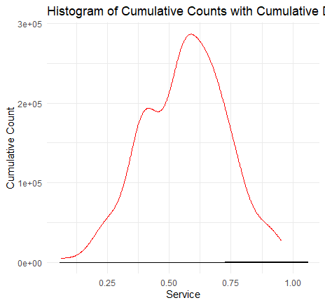
Let's look at the help:
In ?geom_histogram:

Computed variables
These are calculated by the 'stat' part of layers and can be accessed with delayed evaluation.

• after_stat(count)
  number of points in bin.
• after_stat(density)
  density of points in bin, scaled to integrate to 1.
• after_stat(ncount)
  count, scaled to a maximum of 1.
• after_stat(ndensity)
  density, scaled to a maximum of 1.
• after_stat(width)
  widths of bins.

In ?geom_density:

Computed variables
These are calculated by the 'stat' part of layers and can be accessed with delayed evaluation.

• after_stat(density)
  density estimate.
• after_stat(count)
  density * number of points - useful for stacked density plots.
• after_stat(scaled)
  density estimate, scaled to maximum of 1.
• after_stat(n)
  number of points.
• after_stat(ndensity)
  alias for scaled, to mirror the syntax of stat_bin().

So you want both to be on the same scale. In your code, when running geom_histogram(), you take the cumsum of ..count.., which is the number of points in a bin, so the total of that cumsum is the total number of points (the number of rows in data).

We can make that more clear with example data:

library(ggplot2)

set.seed(123)
data <- data.frame(Service = rpois(100, lambda = 1000))

head(data)
#>   Service
#> 1     982
#> 2    1037
#> 3     946
#> 4    1004
#> 5    1054
#> 6    1014

num_bins <- ceiling(1 + log2(nrow(data)))

gg <- ggplot(data, aes(x=Service)) +
  geom_histogram(aes(y=cumsum(..count..)),
                 bins=num_bins, fill="skyblue", color="black")
  
layer_data(gg) |>
  dplyr::select(x, y, count, density, ncount, ndensity)
#> Warning: The dot-dot notation (`..count..`) was deprecated in ggplot2 3.4.0.
#> ℹ Please use `after_stat(count)` instead.
#> This warning is displayed once every 8 hours.
#> Call `lifecycle::last_lifecycle_warnings()` to see where this warning was
#> generated.
#>           x   y count     density     ncount   ndensity
#> 1  941.1429   2     2 0.001147541 0.07142857 0.07142857
#> 2  958.5714   8     6 0.003442623 0.21428571 0.21428571
#> 3  976.0000  26    18 0.010327869 0.64285714 0.64285714
#> 4  993.4286  52    26 0.014918033 0.92857143 0.92857143
#> 5 1010.8571  80    28 0.016065574 1.00000000 1.00000000
#> 6 1028.2857  90    10 0.005737705 0.35714286 0.35714286
#> 7 1045.7143  97     7 0.004016393 0.25000000 0.25000000
#> 8 1063.1429 100     3 0.001721311 0.10714286 0.10714286

^{Created on 2023-12-26 with reprex v2.0.2}

So as you can see here, the maximum of y is 100, which is the number of rows in data, because count contains the number of rows in a bin.

If you want the same scale for the geom_density(), you thus need the maximum to be the number of points, ..n... And you can use a scaled density to make sure the scale is respected:

ggplot(data, aes(x=Service)) +
  geom_histogram(aes(y=cumsum(..count..)),
                 bins=num_bins, fill="skyblue", color="black") +
geom_density(aes(y=..scaled..*..n..), color="red")