Creating a frequency polygon overlay in R

I'm trying to create a frequency polygon overlay plot in R. I have been able to generate relative frequency tables for responses to a 3-question survey, with responses given as discrete values for 1-5.

How can I make a frequency polygon plot that represents the information below (the percent of respondents per event) for multiple events on the same plot?

Here's the dput for the table:

dput(t1)
structure(c(1.33196721311475, 0.867678958785249, 0.995024875621891, 
0.544069640914037, 1.0498687664042, 0, 0.759219088937093, 0.66334991708126, 
0.217627856365615, 0, 1.63934426229508, 6.83297180043384, 0.995024875621891, 
0.870511425462459, 1.0498687664042, 19.5696721311475, 37.0932754880694, 
26.6998341625207, 20.2393906420022, 20.4724409448819, 77.4590163934426, 
54.4468546637744, 70.6467661691542, 78.1284004352557, 77.4278215223097
), .Dim = c(5L, 5L), .Dimnames = structure(list(c("A", "B", "C", 
"D", "E"), c("1", "2", "3", "4", "5")), .Names = c("", "")))

I am also trying to color code the events, so they are differentiated on the resultant plot.

January Events Relative Frequency Table

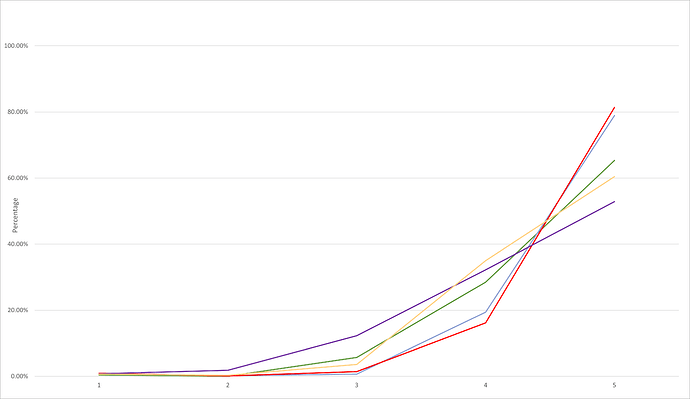
This is what the desired frequency polygon plot would look like (in Excel), however Excel is super inefficient for a task like this, so I thought R could do a better job!
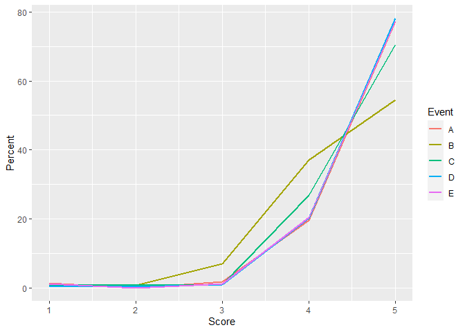
Is this the sort of thing you want to do?

library(tidyr)
library(ggplot2)

t1 <- structure(c(1.33196721311475, 0.867678958785249, 0.995024875621891, 
            0.544069640914037, 1.0498687664042, 0, 0.759219088937093, 0.66334991708126, 
            0.217627856365615, 0, 1.63934426229508, 6.83297180043384, 0.995024875621891, 
            0.870511425462459, 1.0498687664042, 19.5696721311475, 37.0932754880694, 
            26.6998341625207, 20.2393906420022, 20.4724409448819, 77.4590163934426, 
            54.4468546637744, 70.6467661691542, 78.1284004352557, 77.4278215223097
), .Dim = c(5L, 5L), .Dimnames = structure(list(c("A", "B", "C", 
                                                  "D", "E"), c("1", "2", "3", "4", "5")), .Names = c("", "")))
t_trans <- t(t1)
DF <- as.data.frame(t_trans)
DF$Score <- 1:5
DF
#>           A          B          C          D         E Score
#> 1  1.331967  0.8676790  0.9950249  0.5440696  1.049869     1
#> 2  0.000000  0.7592191  0.6633499  0.2176279  0.000000     2
#> 3  1.639344  6.8329718  0.9950249  0.8705114  1.049869     3
#> 4 19.569672 37.0932755 26.6998342 20.2393906 20.472441     4
#> 5 77.459016 54.4468547 70.6467662 78.1284004 77.427822     5


DFlong <- DF |> pivot_longer(cols = -Score,
                             names_to = 'Event')
DFlong
#> # A tibble: 25 x 3
#>    Score Event value
#>    <int> <chr> <dbl>
#>  1     1 A     1.33 
#>  2     1 B     0.868
#>  3     1 C     0.995
#>  4     1 D     0.544
#>  5     1 E     1.05 
#>  6     2 A     0    
#>  7     2 B     0.759
#>  8     2 C     0.663
#>  9     2 D     0.218
#> 10     2 E     0    
#> # ... with 15 more rows
ggplot(DFlong,aes(x = Score, y = value, color = Event)) + 
  geom_line(size=1) + labs(y="Percent")

Created on 2022-03-23 by the reprex package (v2.0.1)

1 Like

This topic was automatically closed 7 days after the last reply. New replies are no longer allowed.

If you have a query related to it or one of the replies, start a new topic and refer back with a link.