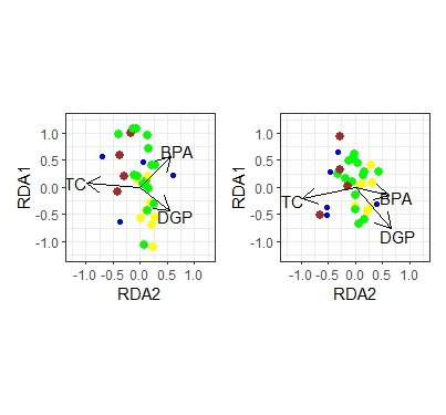
Creating a complete graph from two ordination graphs

Hello,
I am writing to you about a question regarding the grouping of two RDA ordination graphs.
Here is the code of my function that displays correctly and completely for one standard graph: wing<-plot(myrda, display = c("sp", "lc", "cn"), main = "") spe.sc2 <- scores(myrda, choices = 1:2, display = "sp") arrows(0, 0, spe.sc2[, 1] * 0.92, spe.sc2[, 2] * 0.92, length = 0, lty = 1, col = "red")

Then, here is the code to group the two graphs into one: library(repr) par(mfrow = c(1, 1) ) options(repr.plot.width = 16, repr.plot.height = 13)

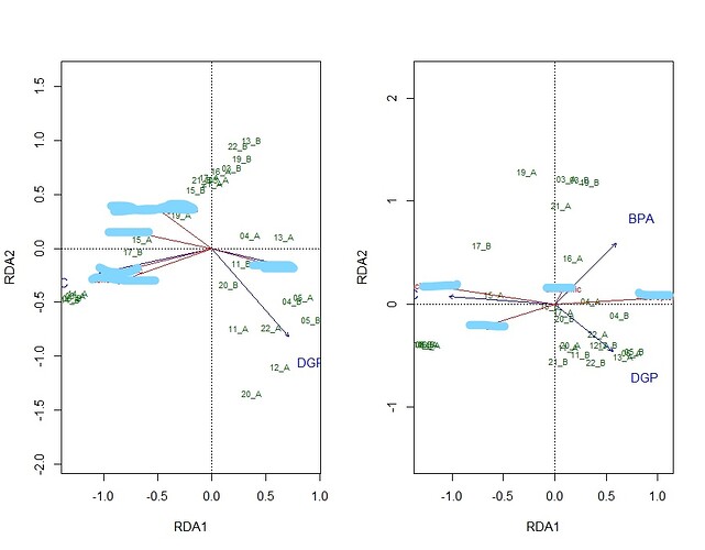
The problem is that the graphs are cut off and some elements aren't visible anymore (blue arrow and red writting). I try to increase the width of the graph with the function "options(repr.plot.width = , repr.plot.height =) " .


(I have hidden the results, as I need to keep some confidentiality with these results, thank you for your understanding.)

But it doesn't solve the problem to get a complete display of the content of my two graphs together. Do you have any idea how to fix the problem?

Thanks in advance for your feedback,
Erwan

The starting point is difficult to replicate without a full a reprex (see the FAQ).. For myrda, use a built-in dataset if you have one to hand or create some fake data. It doesn't matter that the plots may be garbage since all we are trying to do is display side by side without cropping.

Thank you for the answer! Here is a table with the same number of rows and columns but with random numbers.

station	brachypterous	dimorphic	macropterous	wingless	hygrophilic	mesophilic	mesophilic/hygrophilic	xerophilic	steno-hygrophilic	imago	larva	larva/imago	indefinite stage	eurytope	stenotope	e/s	taille_moy	TC	DGP	BPA	Habitats
03_A	80	53	64	59	54	49	15	33	28	20	19	32	33	22	48	4	19	4660	22062	13494	WP
03_B	76	52	11	69	77	78	35	0	8	42	38	23	18	10	21	3	20	1654	22519	16681	WP
04_A	56	70	2	30	19	69	7	20	40	49	28	28	48	44	4	1	9	19106	25111	27239	F
04_B	48	57	59	35	39	32	13	31	40	24	32	13	50	28	33	0	11	26431	1693	20931	NWP
05_A	28	53	14	9	70	77	8	46	19	29	1	26	33	35	14	3	12	13204	10380	18060	NWP
05_B	7	50	76	7	28	21	14	22	11	47	45	28	7	20	5	3	20	24831	22230	2631	NWP
06_A	16	68	2	65	73	30	23	24	17	4	6	26	28	39	0	1	18	17754	24382	23919	F
06_B	10	79	74	63	26	40	34	49	13	14	44	37	14	36	13	1	19	22748	29825	21235	F
11_A	42	67	48	48	39	6	30	16	24	27	6	35	46	25	27	4	14	2163	20859	30760	WP
11_B	74	16	70	3	9	38	4	36	21	11	31	15	47	46	42	3	20	11506	28576	22211	WP
12_A	23	48	62	43	57	56	12	24	37	15	28	34	40	37	2	3	8	3189	9466	17583	WP
12_B	16	53	51	27	12	56	20	20	42	33	30	22	38	13	23	4	17	4757	6049	28510	WP
13_A	52	42	17	30	34	40	16	28	34	18	18	20	25	32	15	5	15	27349	15330	18622	NWP
13_B	62	2	67	35	25	77	43	20	5	5	41	45	31	5	50	2	13	30400	19374	11243	NWP
14_A	79	71	29	34	43	77	10	4	39	2	47	41	29	3	5	1	8	3196	6623	4379	F
14_B	74	20	64	57	8	79	32	31	8	36	41	11	24	31	10	5	17	14038	3310	13354	F
15_A	76	53	2	57	59	39	40	32	28	26	8	12	33	19	29	1	14	184	1398	18665	WP
15_B	58	64	58	10	72	41	37	39	24	24	12	4	23	34	48	5	8	9439	18474	3927	WP
16_A	26	18	61	65	55	14	8	27	33	26	25	6	33	47	45	3	14	4064	24519	6417	WP
17_A	16	75	79	7	15	52	32	48	39	25	16	28	3	32	13	2	12	6883	19115	11786	WP
17_B	72	74	18	21	23	69	31	8	11	31	1	25	30	32	31	5	8	24972	26490	7016	F
19_A	44	34	63	64	58	54	40	47	50	13	24	21	17	7	43	2	16	25949	10927	8220	F
19_B	27	6	71	12	61	27	34	4	47	17	35	49	45	21	25	5	8	30463	26925	25047	F
20_A	73	18	43	29	49	61	42	23	11	29	19	47	8	34	48	2	11	16279	29764	16044	WP
20_B	33	20	50	35	45	33	14	45	20	47	34	34	43	49	0	0	20	19937	3501	23967	WP
21_A	66	13	11	66	41	69	33	3	0	36	50	3	45	42	42	4	20	16327	21676	9521	F
21_B	55	20	34	27	41	53	6	9	10	41	48	10	38	24	19	5	14	5295	20168	22494	F
22_A	34	51	3	4	57	38	27	26	32	21	37	15	4	3	20	3	14	6986	28462	27038	NWP
22_B	6	44	50	54	76	78	21	48	42	18	41	8	46	38	17	5	15	11457	20345	18741	NWP

Here are the full lines of code to create the two plots:

names(trait_ecolo_abondance_var_env)
Y = trait_ecolo_abondance_var_env[, c(1:4)]; summary(Y)

pairs(Y, panel=panel.smooth)
X = trait_ecolo_abondance_var_env[, c(18,19,20)]; summary(X)
pairs(X, panel=panel.smooth)

myrda <- rda(log(Y[-12,]+1) ~ TC + DGP + BPA, scale=TRUE, data=trait_ecolo_abondance_var_env[-12,])
anova(myrda, by="terms")
summary(myrda)

# Plot of Scaling 2
wing<-plot(myrda,
     display = c("sp", "lc", "cn"),
     main = "")
spe.sc2 <- scores(myrda,
                  choices = 1:2,
                  display = "sp")
arrows(0, 0,
       spe.sc2[, 1] * 0.92,
       spe.sc2[, 2] * 0.92,
       length = 0,
       lty = 1, col = "red")

#################################

Y1 = trait_ecolo_abondance_var_env[, c(5:9)]; summary(Y1)

pairs(Y1, panel=panel.smooth)
X1 = trait_ecolo_abondance_var_env[, c(18,19,20)]; summary(X1)
pairs(X1, panel=panel.smooth)

myrda1 <- rda(log(Y1[-12,]+1) ~ TC + DGP + BPA, scale=TRUE, data=trait_ecolo_abondance_var_env[-12,])
anova(myrda1, by="terms")
summary(myrda1)
# Plot of Scaling 2
moisture<-plot(myrda1,
     display = c("sp", "lc", "cn"),
     main = "")
spe.sc21 <- scores(myrda1,
                   choices = 1:2,
                   display = "sp")
arrows(0, 0,
       spe.sc21[, 1] * 0.92,
       spe.sc21[, 2] * 0.92,
       length = 0,
       lty = 1, col = "red")

Now all I need to do is put the moisture and wing plots together, so that everything is displayed completely. If you can help me, that would be great!

The reprex won't render, so I'm only attaching the final side-by-side plots. I'm unsure what it is that needs to be changed, however.

library(vegan)
d <- data.frame(
  station = c(
    "03_A", "03_B", "04_A", "04_B", "05_A",
    "05_B", "06_A", "06_B", "11_A", "11_B", "12_A", "12_B", "13_A",
    "13_B", "14_A", "14_B", "15_A", "15_B", "16_A", "17_A", "17_B",
    "19_A", "19_B", "20_A", "20_B", "21_A", "21_B", "22_A", "22_B"
  ), brachypterous = c(
    80, 76, 56, 48, 28, 7, 16, 10, 42,
    74, 23, 16, 52, 62, 79, 74, 76, 58, 26, 16, 72, 44,
    27, 73, 33, 66, 55, 34, 6
  ), dimorphic = c(
    53, 52, 70,
    57, 53, 50, 68, 79, 67, 16, 48, 53, 42, 2, 71, 20,
    53, 64, 18, 75, 74, 34, 6, 18, 20, 13, 20, 51, 44
  ), macropterous = c(
    64, 11, 2, 59, 14, 76, 2, 74, 48,
    70, 62, 51, 17, 67, 29, 64, 2, 58, 61, 79, 18, 63,
    71, 43, 50, 11, 34, 3, 50
  ), wingless = c(
    59, 69, 30,
    35, 9, 7, 65, 63, 48, 3, 43, 27, 30, 35, 34, 57,
    57, 10, 65, 7, 21, 64, 12, 29, 35, 66, 27, 4, 54
  ), hygrophilic = c(
    54, 77, 19, 39, 70, 28, 73, 26, 39,
    9, 57, 12, 34, 25, 43, 8, 59, 72, 55, 15, 23, 58,
    61, 49, 45, 41, 41, 57, 76
  ), mesophilic = c(
    49, 78,
    69, 32, 77, 21, 30, 40, 6, 38, 56, 56, 40, 77, 77,
    79, 39, 41, 14, 52, 69, 54, 27, 61, 33, 69, 53, 38,
    78
  ), mesophilic_hygrophilic = c(
    15, 35, 7, 13, 8, 14,
    23, 34, 30, 4, 12, 20, 16, 43, 10, 32, 40, 37, 8,
    32, 31, 40, 34, 42, 14, 33, 6, 27, 21
  ), xerophilic = c(
    33,
    0, 20, 31, 46, 22, 24, 49, 16, 36, 24, 20, 28, 20,
    4, 31, 32, 39, 27, 48, 8, 47, 4, 23, 45, 3, 9, 26,
    48
  ), steno_hygrophilic = c(
    28, 8, 40, 40, 19, 11, 17,
    13, 24, 21, 37, 42, 34, 5, 39, 8, 28, 24, 33, 39,
    11, 50, 47, 11, 20, 0, 10, 32, 42
  ), imago = c(
    20, 42,
    49, 24, 29, 47, 4, 14, 27, 11, 15, 33, 18, 5, 2,
    36, 26, 24, 26, 25, 31, 13, 17, 29, 47, 36, 41, 21,
    18
  ), larva = c(
    19, 38, 28, 32, 1, 45, 6, 44, 6, 31,
    28, 30, 18, 41, 47, 41, 8, 12, 25, 16, 1, 24, 35,
    19, 34, 50, 48, 37, 41
  ), larva_imago = c(
    32, 23, 28,
    13, 26, 28, 26, 37, 35, 15, 34, 22, 20, 45, 41, 11,
    12, 4, 6, 28, 25, 21, 49, 47, 34, 3, 10, 15, 8
  ),
  indefinite.stage = c(
    33, 18, 48, 50, 33, 7, 28, 14,
    46, 47, 40, 38, 25, 31, 29, 24, 33, 23, 33, 3,
    30, 17, 45, 8, 43, 45, 38, 4, 46
  ), eurytope = c(
    22,
    10, 44, 28, 35, 20, 39, 36, 25, 46, 37, 13, 32,
    5, 3, 31, 19, 34, 47, 32, 32, 7, 21, 34, 49,
    42, 24, 3, 38
  ), stenotope = c(
    48, 21, 4, 33, 14,
    5, 0, 13, 27, 42, 2, 23, 15, 50, 5, 10, 29, 48,
    45, 13, 31, 43, 25, 48, 0, 42, 19, 20, 17
  ), e_s = c(
    4,
    3, 1, 0, 3, 3, 1, 1, 4, 3, 3, 4, 5, 2, 1, 5,
    1, 5, 3, 2, 5, 2, 5, 2, 0, 4, 5, 3, 5
  ), taille_moy = c(
    19,
    20, 9, 11, 12, 20, 18, 19, 14, 20, 8, 17, 15,
    13, 8, 17, 14, 8, 14, 12, 8, 16, 8, 11, 20, 20,
    14, 14, 15
  ), TC = c(
    4660, 1654, 19106, 26431, 13204,
    24831, 17754, 22748, 2163, 11506, 3189, 4757, 27349,
    30400, 3196, 14038, 184, 9439, 4064, 6883, 24972,
    25949, 30463, 16279, 19937, 16327, 5295, 6986, 11457
  ), DGP = c(
    22062, 22519, 25111, 1693, 10380, 22230,
    24382, 29825, 20859, 28576, 9466, 6049, 15330, 19374,
    6623, 3310, 1398, 18474, 24519, 19115, 26490, 10927,
    26925, 29764, 3501, 21676, 20168, 28462, 20345
  ), BPA = c(
    13494,
    16681, 27239, 20931, 18060, 2631, 23919, 21235, 30760,
    22211, 17583, 28510, 18622, 11243, 4379, 13354, 18665,
    3927, 6417, 11786, 7016, 8220, 25047, 16044, 23967,
    9521, 22494, 27038, 18741
  ), Habitats = c(
    "WP", "WP",
    "F", "NWP", "NWP", "NWP", "F", "F", "WP", "WP", "WP", "WP",
    "NWP", "NWP", "F", "F", "WP", "WP", "WP", "WP", "F", "F",
    "F", "WP", "WP", "F", "F", "NWP", "NWP"
  )
)

# omitted non-numeric variable station
Y <- d[, c(2:4)]
summary(Y)

pairs(Y, panel = panel.smooth)

X <- d[, c(18, 19, 20)]
summary(X)
pairs(X, panel = panel.smooth)

myrda <- rda(log(Y[-12, ] + 1) ~ TC + DGP + BPA, scale = TRUE, data = d[-12, ])
anova(myrda, by = "terms")
summary(myrda)

# Plot of Scaling 2
# wing <- plot(myrda,
#   display = c("sp", "lc", "cn"),
#   main = ""
# )
spe.sc2 <- scores(myrda,
  choices = 1:2,
  display = "sp"
)
arrows(0, 0,
  spe.sc2[, 1] * 0.92,
  spe.sc2[, 2] * 0.92,
  length = 0,
  lty = 1, col = "red"
)

#################################

Y1 <- d[, c(5:9)]
summary(Y1)

pairs(Y1, panel = panel.smooth)
X1 <- d[, c(18, 19, 20)]
summary(X1)
pairs(X1, panel = panel.smooth)

myrda1 <- rda(log(Y1[-12, ] + 1) ~ TC + DGP + BPA, scale = TRUE, data = d[-12, ])
anova(myrda1, by = "terms")
summary(myrda1)
# Plot of Scaling 2
moisture <- plot(myrda1,
  display = c("sp", "lc", "cn"),
  main = ""
)
spe.sc21 <- scores(myrda1,
  choices = 1:2,
  display = "sp"
)
arrows(0, 0,
  spe.sc21[, 1] * 0.92,
  spe.sc21[, 2] * 0.92,
  length = 0,
  lty = 1, col = "red"
)

par(mfrow = c(1,2))
plot(myrda,display = c("sp", "lc", "cn"))
plot(myrda1,display = c("sp", "lc", "cn"))
dev.off()

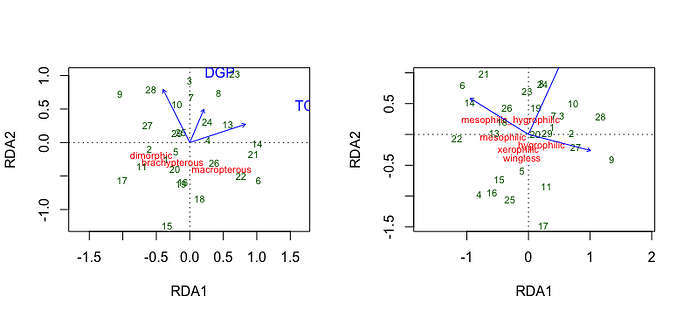
Thank you for your feedback and patience! This is exactly the kind of combined graph I want. But the problem is that the display of environmental variables like TC, BPA are cut off or not visible in my final case. Same problem for explanatory variables like macropterous or hygrophilic, which are not or only half displayed in the combined plot.

So, how to bring closer the writings of the blue and red variables, so that they all appear on the combined plot?

OK, I see the problem now. When plotted singly, the name displays are ok, but squeezing them into a single graphic, either horizontally or vertically doesn't. I guess the next question is what is the target document for this illustration and the page layout constraint?

Yes exactly, your summary is right.
Indeed, I am looking for a way to display the names and variables entirely while compressing them into a single graph. Is there a possibility on R or should I look at other software to merge two figures into one without losing quality ?

The way to try to fix this depends on if the output will be HTML or pdf. (If it's in Word, I can't help.) Do you use LaTeX?

I don't really know what Latex is. I think it will be rather pdf. I've already tried merging my two graphics in freeware, but the quality drops too much. I'm a bit lost and stuck with this situation. Do you have an idea in mind or an avenue to explore? Thanks for your help!

LsTeX is a typesetting program widely used in academic publishing, including graduate theses and dissertations. It uses mark-up conventions that that are capable of placing high resolution text and images anywhere on the page. It comes, however, at the cost of a learning curve that is much steeper than R. No one is likely to pick it up as a "nice to have, only as a must have. The low-level representation used is TeX, which is produced under the hood by Rmarkdown through a behind the scenes program pandoc as an intermediate step in producing a pdf output. For the fullest possible control, there's an option to save and edit that intermediate output. I can't recommend it. For more limited tweaking, RMarkdown will accept higher-level LaTeX markup or HTML, but not in the same document.

Let me try to come up with an example using pdf as a target. Ping me with a DM after a decent interval. It's after 4AM, so it's time for me to nod off.

Found a {ggplot2} solution that will solve the basic problem. I don't know how much embellishment you need in terms of labels, light weight, color, title, caption, font, etc.

# Install the package as follows:

# Enable the r-universe repo
options(repos = c(
  fawda123 = 'https://fawda123.r-universe.dev',
  CRAN = 'https://cloud.r-project.org'))

# install.packages("ggord") first
library(ggord)
library(ggplot2)
library(patchwork)
library(scales)
library(vegan)
#> Loading required package: permute
#> Loading required package: lattice
#> This is vegan 2.6-4

d <- data.frame(
  station = c(
    "03_A", "03_B", "04_A", "04_B", "05_A",
    "05_B", "06_A", "06_B", "11_A", "11_B", "12_A", "12_B", "13_A",
    "13_B", "14_A", "14_B", "15_A", "15_B", "16_A", "17_A", "17_B",
    "19_A", "19_B", "20_A", "20_B", "21_A", "21_B", "22_A", "22_B"
  ), brachypterous = c(
    80, 76, 56, 48, 28, 7, 16, 10, 42,
    74, 23, 16, 52, 62, 79, 74, 76, 58, 26, 16, 72, 44,
    27, 73, 33, 66, 55, 34, 6
  ), dimorphic = c(
    53, 52, 70,
    57, 53, 50, 68, 79, 67, 16, 48, 53, 42, 2, 71, 20,
    53, 64, 18, 75, 74, 34, 6, 18, 20, 13, 20, 51, 44
  ), macropterous = c(
    64, 11, 2, 59, 14, 76, 2, 74, 48,
    70, 62, 51, 17, 67, 29, 64, 2, 58, 61, 79, 18, 63,
    71, 43, 50, 11, 34, 3, 50
  ), wingless = c(
    59, 69, 30,
    35, 9, 7, 65, 63, 48, 3, 43, 27, 30, 35, 34, 57,
    57, 10, 65, 7, 21, 64, 12, 29, 35, 66, 27, 4, 54
  ), hygrophilic = c(
    54, 77, 19, 39, 70, 28, 73, 26, 39,
    9, 57, 12, 34, 25, 43, 8, 59, 72, 55, 15, 23, 58,
    61, 49, 45, 41, 41, 57, 76
  ), mesophilic = c(
    49, 78,
    69, 32, 77, 21, 30, 40, 6, 38, 56, 56, 40, 77, 77,
    79, 39, 41, 14, 52, 69, 54, 27, 61, 33, 69, 53, 38,
    78
  ), mesophilic_hygrophilic = c(
    15, 35, 7, 13, 8, 14,
    23, 34, 30, 4, 12, 20, 16, 43, 10, 32, 40, 37, 8,
    32, 31, 40, 34, 42, 14, 33, 6, 27, 21
  ), xerophilic = c(
    33,
    0, 20, 31, 46, 22, 24, 49, 16, 36, 24, 20, 28, 20,
    4, 31, 32, 39, 27, 48, 8, 47, 4, 23, 45, 3, 9, 26,
    48
  ), steno_hygrophilic = c(
    28, 8, 40, 40, 19, 11, 17,
    13, 24, 21, 37, 42, 34, 5, 39, 8, 28, 24, 33, 39,
    11, 50, 47, 11, 20, 0, 10, 32, 42
  ), imago = c(
    20, 42,
    49, 24, 29, 47, 4, 14, 27, 11, 15, 33, 18, 5, 2,
    36, 26, 24, 26, 25, 31, 13, 17, 29, 47, 36, 41, 21,
    18
  ), larva = c(
    19, 38, 28, 32, 1, 45, 6, 44, 6, 31,
    28, 30, 18, 41, 47, 41, 8, 12, 25, 16, 1, 24, 35,
    19, 34, 50, 48, 37, 41
  ), larva_imago = c(
    32, 23, 28,
    13, 26, 28, 26, 37, 35, 15, 34, 22, 20, 45, 41, 11,
    12, 4, 6, 28, 25, 21, 49, 47, 34, 3, 10, 15, 8
  ),
  indefinite.stage = c(
    33, 18, 48, 50, 33, 7, 28, 14,
    46, 47, 40, 38, 25, 31, 29, 24, 33, 23, 33, 3,
    30, 17, 45, 8, 43, 45, 38, 4, 46
  ), eurytope = c(
    22,
    10, 44, 28, 35, 20, 39, 36, 25, 46, 37, 13, 32,
    5, 3, 31, 19, 34, 47, 32, 32, 7, 21, 34, 49,
    42, 24, 3, 38
  ), stenotope = c(
    48, 21, 4, 33, 14,
    5, 0, 13, 27, 42, 2, 23, 15, 50, 5, 10, 29, 48,
    45, 13, 31, 43, 25, 48, 0, 42, 19, 20, 17
  ), e_s = c(
    4,
    3, 1, 0, 3, 3, 1, 1, 4, 3, 3, 4, 5, 2, 1, 5,
    1, 5, 3, 2, 5, 2, 5, 2, 0, 4, 5, 3, 5
  ), taille_moy = c(
    19,
    20, 9, 11, 12, 20, 18, 19, 14, 20, 8, 17, 15,
    13, 8, 17, 14, 8, 14, 12, 8, 16, 8, 11, 20, 20,
    14, 14, 15
  ), TC = c(
    4660, 1654, 19106, 26431, 13204,
    24831, 17754, 22748, 2163, 11506, 3189, 4757, 27349,
    30400, 3196, 14038, 184, 9439, 4064, 6883, 24972,
    25949, 30463, 16279, 19937, 16327, 5295, 6986, 11457
  ), DGP = c(
    22062, 22519, 25111, 1693, 10380, 22230,
    24382, 29825, 20859, 28576, 9466, 6049, 15330, 19374,
    6623, 3310, 1398, 18474, 24519, 19115, 26490, 10927,
    26925, 29764, 3501, 21676, 20168, 28462, 20345
  ), BPA = c(
    13494,
    16681, 27239, 20931, 18060, 2631, 23919, 21235, 30760,
    22211, 17583, 28510, 18622, 11243, 4379, 13354, 18665,
    3927, 6417, 11786, 7016, 8220, 25047, 16044, 23967,
    9521, 22494, 27038, 18741
  ), Habitats = c(
    "WP", "WP",
    "F", "NWP", "NWP", "NWP", "F", "F", "WP", "WP", "WP", "WP",
    "NWP", "NWP", "F", "F", "WP", "WP", "WP", "WP", "F", "F",
    "F", "WP", "WP", "F", "F", "NWP", "NWP"
  )
)

# omitted non-numeric variable station
Y <- d[, c(2:4)]
# summary(Y)

# pairs(Y, panel = panel.smooth)

X <- d[, c(18, 19, 20)]
# summary(X)
# pairs(X, panel = panel.smooth)

myrda <- rda(log(Y[-12, ] + 1) ~ TC + DGP + BPA, scale = TRUE, data = d[-12, ])
# anova(myrda, by = "terms")
# summary(myrda)

# Plot of Scaling 2
# wing <- plot(myrda,
#   display = c("sp", "lc", "cn"),
#   main = ""
# )
# spe.sc2 <- scores(myrda,
#                   choices = 1:2,
#                   display = "sp"
# )
# arrows(0, 0,
#        spe.sc2[, 1] * 0.92,
#        spe.sc2[, 2] * 0.92,
#        length = 0,
#        lty = 1, col = "red"
# )

#################################

Y1 <- d[, c(5:9)]
# summary(Y1)

# pairs(Y1, panel = panel.smooth)
X1 <- d[, c(18, 19, 20)]
# summary(X1)
# pairs(X1, panel = panel.smooth)

myrda1 <- rda(log(Y1[-12, ] + 1) ~ TC + DGP + BPA, scale = TRUE, data = d[-12, ])
# anova(myrda1, by = "terms")
# summary(myrda1)
# Plot of Scaling 2
# moisture <- plot(myrda1,
#                  display = c("sp", "lc", "cn"),
#                  main = ""
# )
# spe.sc21 <- scores(myrda1,
#                    choices = 1:2,
#                    display = "sp"
# )
# arrows(0, 0,
#        spe.sc21[, 1] * 0.92,
#        spe.sc21[, 2] * 0.92,
#        length = 0,
#        lty = 1, col = "red"
# )
# plot.new()

# par(mfrow = c(1,2))
# plot(myrda,display = c("sp", "lc", "cn"))
# plot(myrda1,display = c("sp", "lc", "cn"))
# dev.off()

s <- summary(myrda)$concont$importance
s_x <- paste0("RDA2 (",percent(s[2], .01),")")
s_y <- paste0("RDA1 (",percent(s[5], .01),")")
s1 <- summary(myrda)$concont$importance
s1_x <- paste0("RDA2 (",percent(s[2], .01),")")
s1_y <- paste0("RDA1 (",percent(s[5], .01),")")

left <- ggord(myrda) +
  xlim(-1.25,1.25) +
  ylim(-1.25,1.25) +
  xlab(s_x) +
  ylab(s_y)
#> Scale for x is already present.
#> Adding another scale for x, which will replace the existing scale.
#> Scale for y is already present.
#> Adding another scale for y, which will replace the existing scale.
right <- ggord(myrda1) +
  xlim(-1.25,1.25) +
  ylim(-1.25,1.25) +
  xlab(s1_x) +
  ylab(s1_y)
#> Scale for x is already present.
#> Adding another scale for x, which will replace the existing scale.
#> Scale for y is already present.
#> Adding another scale for y, which will replace the existing scale.
left + right
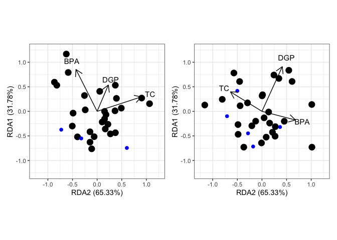
Created on 2023-05-25 with reprex v2.0.2
Great, thanks for the progress!
I am getting closer to the solution. I still have some aesthetic questions for this graphic:

  • How do you turn the black dots into green study site names (e.g. 03_A, 11_B)? Like in the first graphs sent in this discussion.
  • How to replace the blue dots by red arrows named by the response variables in red (hygrophilic or brachypterous, etc)?
  • Can we remove the percentage in the x- and y-axis and keep only RDA 1 and RDA2?
  • How can the colour of the arrows and texts of the explanatory variables (TC, DGP, SPB) be changed from black to blue?

Thank you again for your time and energy :slight_smile: !

I'm sure this can all be done, but requires some excavation into the objects.

  1. Dot labels: we need first to examine the rda objects to see where the d$station variable gets mapped—that's a matter of str(myrda) to see where it's tucked away.

  2. Blue dots/response variable names. Depends on whether this will be a recurring use, in which case it should be done programmatically and digging out where it's located within the rda object is again necessary. Or, it can be hardwired by hand and put down as geom_text objects. I don't understand red arrows, however. I assumed you'd want the existing black arrows recolored.

  3. axes: just need to adjust s_x s_y s1_x s2_y definitions.

  4. To change colors and line weights will require me to tinker with the ggnorm definition to see where to adjust. Shouldn't be too hard.

Why don't you get back to me with #1 & 2, digging through str(myrda)? #3 is trivial and I'll take #4.

Hello,

Thank you for your reply! Sorry for my late reply, I've been working a lot on my job lately and unfortunately have less time for statistics. Nevertheless, I've made as much progress as I can, but I'm still stuck on certain points. I can hardly find any examples in ggord to inspire me.

That said, I have found a fairly simple way of merging two graphs together using the :

layout(matrix(1:2,1,2))

Then, when exporting the image, I vary the height and width so that everything appears on the plot. It's doable, but the text is still very small and it's a bit of a DIY job.

As for my 4 questions:

I succeeded with point #3, which was fairly easy.

For point #1, I tried using geom_text with label=station. But that didn't work. Besides, I don't see how the str() function can help me. Another hint would be welcome :-).

For point #2, I tried digging around with the ggord arrow() function. But I don't think I'm on the right track. Do you have another idea or again what information can str() give me?

I've made one improvement though: I've coloured the points in the ordering by habitat, which adds to understanding. Here's the code so far :

s <- summary(myrda)$concont$importance
s_x <- paste0("RDA2")
s_y <- paste0("RDA1")
s1 <- summary(myrda1)$concont$importance
s1_x <- paste0("RDA2")
s1_y <- paste0("RDA1")

left<- ggord(myrda,trait_ecolo_abondance_var_env[-12,]$Habitats,ellipse=F,size=2.5,) +
  xlim(-1.25,1.25) +
  ylim(-1.25,1.25) +
  xlab(s_x) +
  ylab(s_y)+
  theme(legend.position="none")+
  scale_colour_manual(values = c("brown","yellow","green")) 
left

#doesn't work: geom_text(aes(label=trait_ecolo_abondance_var_env[-12]$station.1),size=3,check_overlap = TRUE, vjust=-1)

right <- ggord(myrda1,trait_ecolo_abondance_var_env[-12,]$Habitats,ellipse=F,size=2.5)+
  xlim(-1.25,1.25) +
  ylim(-1.25,1.25) +
  xlab(s1_x) +
  ylab(s1_y)+
  theme(legend.position="none")+
  scale_colour_manual(values = c("brown","yellow","green"))
right
left+right

Rplot24

As I said, I'm always interested in new hints or examples that I can use as inspiration.

Thank you and best regards,
Erwan Zimmermann

sty(myrda)
...
rownames(myrda$CCA$v)
#[1] "brachypterous" "dimorphic"     "macropterous" 

Looking at the structure of the rda objects allows seeing where to extract elements needed to add to plot.

Still need help on #4, colors and lineweights?

Everything's in order for point 4. In the image, I succeeded in doing this. With this code :

sites.long2 <- sites.long(plot2, env.data=dune.env)#code to create arrow 
plot2 <- ordiplot(myrda, choices=c(1,2))
species.long2 <- species.long(plot2)
species.long2
species.long2 <- species.long(plot2, spec.data=dune.env)
species.long2

ggord(myrda,trait_ecolo_abondance_var_env[-12,]$Habitats,ellipse=F, ptslab=T,addsize = 6/2) +
  xlim(-1.25,1.25) +
  ylim(-1.25,1.25) +
  xlab(s_x) +
  ylab(s_y)+
  theme(legend.position="none")+
  scale_colour_manual(values = c("brown","yellow","green"))+
  geom_text(
    aes(label = row.names(myrda$CA$u)))+
  geom_segment(data=species.long2, aes(x=1, y=0, xend=axis1*4, yend=axis2*4), 
  colour="red", size=0.7, arrow=arrow())

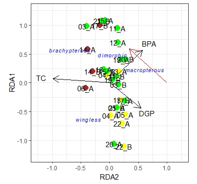
Rplot04

Now I'd just like to connect the names brachypterous, wingless, etc. with arrows. I saw that you could do this with geom_segment, which I've done with this red arrow linked to nothing in the image. Am I going in the right direction? Or what would you advise me to do?

Thanks in advance!

I don't understand what is being illustrated. Just highlighting the location of the label? Otherwise, what is the origin destination?

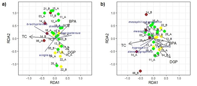
I answered my own question about the arrows. I wanted the arrows to start from the centre (0;0) and reach the names brachypterous, wingless and so on. It's a bit tinkering, but I used this code:

s <- summary(myrda)$concont$importance ; s
s_x <- paste0("RDA1")
s_y <- paste0("RDA2")
s1 <- summary(myrda1)$concont$importance
s1_x <- paste0("RDA1")
s1_y <- paste0("RDA2")
myrda$CA$u

dune.env<-trait_ecolo_abondance_var_env[,18:21][-12,]

plot2 <- ordiplot(myrda, choices=c(1,2))
sites.long2 <- sites.long(plot2, env.data=dune.env)#code to create arrow 
sites.long2
species.long2 <- species.long(plot2)
species.long2
species.long3 <- species.long(plot2, spec.data=dune.env)
species.long3

left<-ggord(myrda,trait_ecolo_abondance_var_env[-12,]$Habitats,ellipse=F, ptslab=T,addsize = 6/2) +
  xlim(-1.3,1.3) +
  ylim(-1.3,1.3) +
  xlab(s_x) +
  ylab(s_y)+
  theme(legend.position="none")+
  scale_colour_manual(values = c("brown","yellow","green"))+
  geom_text_repel(aes(label = row.names(myrda$CA$u)),size = 3) +
  geom_segment(data=species.long2, aes(x=0, y=0, xend=-0.8 , yend=0.47), 
  colour="blue", size=0.5,arrow = arrow(length = unit(0, "cm")))+
  geom_segment(data=species.long2, aes(x=0, y=0, xend=0.075 , yend=0.36), 
               colour="blue", size=0.5,arrow = arrow(length = unit(0, "cm")))+
  geom_segment(data=species.long2, aes(x=0, y=0, xend=0.65 , yend=0.125), 
               colour="blue", size=0.5,arrow = arrow(length = unit(0, "cm")))+
  geom_segment(data=species.long2, aes(x=0, y=0, xend=-0.4 , yend=-0.52), 
               colour="blue", size=0.5,arrow = arrow(length = unit(0, "cm")))
left

right <- ggord(myrda1,trait_ecolo_abondance_var_env[-12,]$Habitats,ellipse=F, ptslab=T,addsize = 6/2)+
  xlim(-1.3,1.3) +
  ylim(-1.3,1.3) +
  xlab(s1_x) +
  ylab(s1_y)+
  theme(legend.position="none")+
  scale_colour_manual(values = c("brown","yellow","green"))+
  geom_text_repel(aes(label = row.names(myrda1$CA$u)),size = 3) +
  geom_segment(data=species.long2, aes(x=0, y=0, xend=-0.45 , yend=0.24), 
               colour="blue", size=0.5,arrow = arrow(length = unit(0, "cm")))+
  geom_segment(data=species.long2, aes(x=0, y=0, xend=-0.29 , yend=0.58), 
               colour="blue", size=0.5,arrow = arrow(length = unit(0, "cm")))+
  geom_segment(data=species.long2, aes(x=0, y=0, xend=0.4 , yend=-0.25), 
               colour="blue", size=0.5,arrow = arrow(length = unit(0, "cm")))+
  geom_segment(data=species.long2, aes(x=0, y=0, xend=-0.585 , yend=-0.485), 
               colour="blue", size=0.5,arrow = arrow(length = unit(0, "cm")))+
  geom_segment(data=species.long2, aes(x=0, y=0, xend=-0.51 , yend=-0.279), 
               colour="blue", size=0.5,arrow = arrow(length = unit(0, "cm")))
right
left+right
plot_grid(left, right, labels=c("a)", "b)"), ncol = 2, nrow = 1)

As for the customization, I succeeded in doing what I wanted. So it succeeded! Unfortunately, I noticed that one point was not being displayed in the graph A, 06_B. The following error messages were displayed:

Removed 1 rows containing missing values (geom_point()).
Removed 1 rows containing missing values (geom_text_repel()).

It's really difficult, I thought I'd done the hard part. I don't understand why a point isn't displayed... it's enough to make you tear your hair out...
It says that there are missing values with 06_B, but that's not true, nothing is missing.
I did notice, however, that when I used the species.long() function to determine the coordinates of axes 1 and 2, the wingless variable and site 06_B had the same coordinates (see photos). Is there a problem here? What do you do when this kind of thing happens?
InkedCapture

I'll need to retrace my step and then follow you here to weight in. Ping me after a decent interval if you don't see anything.

Sorry, unable to reproduce without a complete reprex because there are several missing objects.