Create interactive map for Perú

[Atalaveracuya]

database download: https://we.tl/t-tNYx6Crbag

# Mapa interactivo con R

library(plotly)
df <- read.csv("H:/GRAFICAS INTERACTIVAS/Ejemplo_32-mapa/muertes.csv")
df$hover <- with(df, paste(depart, '<br>', "Muertes", muertes2018, "Fetales %", pcfet2018, "<br>",
                           "Neonatos %", pcneo2018))

# Dar a los límites departamentales un color blanco
l <- list(color = toRGB("white"), width = 2)

# specify some map projection/options
g <- list(
  scope = 'peru',
  projection = list(type = 'mercator'),
  showlakes = TRUE,
  lakecolor = toRGB('white')
)



p <- plot_geo(df, locationmode = 'peru') %>%
  add_trace(
    z = ~muertes2018, text = ~muertes2018, locations = ~dpto,
    color = ~muertes2018, colors = 'Purples'
  ) %>%
  colorbar(title = "Muertes 2018 (fetales y neonatos)") %>%
  layout(
    title = '2018 PERU Muertes por departamento<br>(Fetales y neonatales)',
    geo = g
  )

p

[andresrcs]

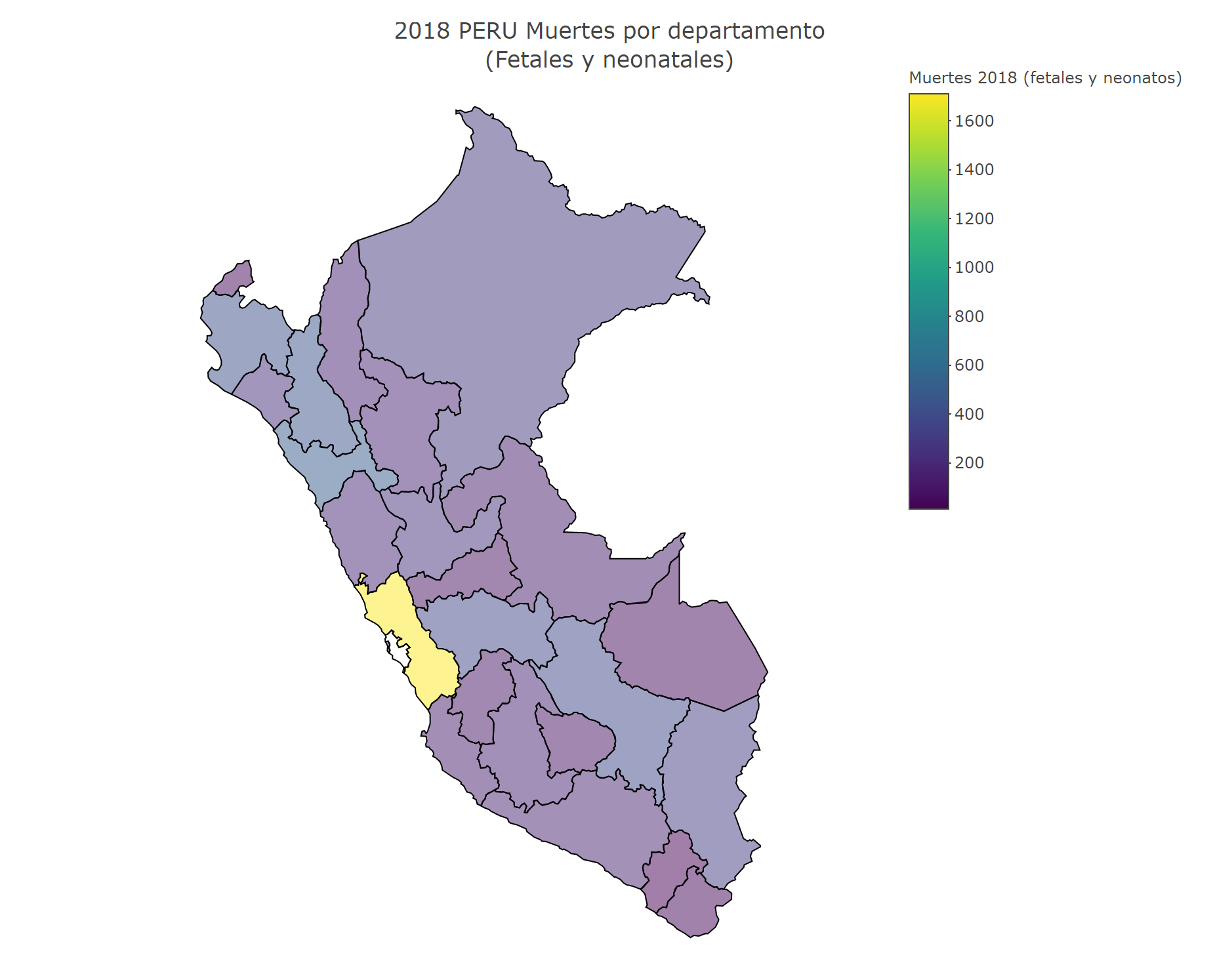
The last time I checked, plotly only provided state level polygons for the U.S., so if you want to make a choropleth for Perú you need to provide your own polygons, I can share with you a light department level sf file you can work with, see this example:

library(tidyverse)
library(plotly)

mapa_peru <- readRDS("peru_simp.rds")
df <- read.csv("muertes.csv")

names <- c("Apur.+" = "Apurímac", "Huánuco" = "Huánuco", "Junin" = "Junín", "San Martin" = "San Martín")

map_data <- df %>% 
    mutate(depart = str_replace_all(depart, names),
           hover = paste(depart, '<br>', "Muertes", muertes2018, "Fetales %", pcfet2018, "<br>",
                         "Neonatos %", pcneo2018)) %>% 
    full_join(mapa_peru, by = c("depart" = "NAME_1"))
map_data <- sf::st_sf(map_data)

plot_ly(map_data, color = I("gray90"), stroke = I("black"), span = I(1)) %>% 
    add_sf(
        color = ~muertes2018, 
        split = ~depart, 
        span = I(1),
        text = ~hover,
        hoverinfo = "text",
        hoveron = "fills"
    ) %>%
    colorbar(title = "Muertes 2018 (fetales y neonatos)") %>%
    layout(
        title = '2018 PERU Muertes por departamento<br>(Fetales y neonatales)',
        showlegend = FALSE
    )

[Atalaveracuya]

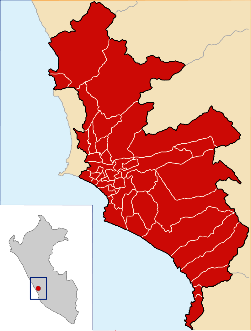
Muchas gracias Andrés. Dime, ¿El área pequeña es Lima metropolitana?. Si fuera Lima Metropolitana estaría compuesta por la provincia de Lima y la prov. constitucional del Callao.

[andresrcs]

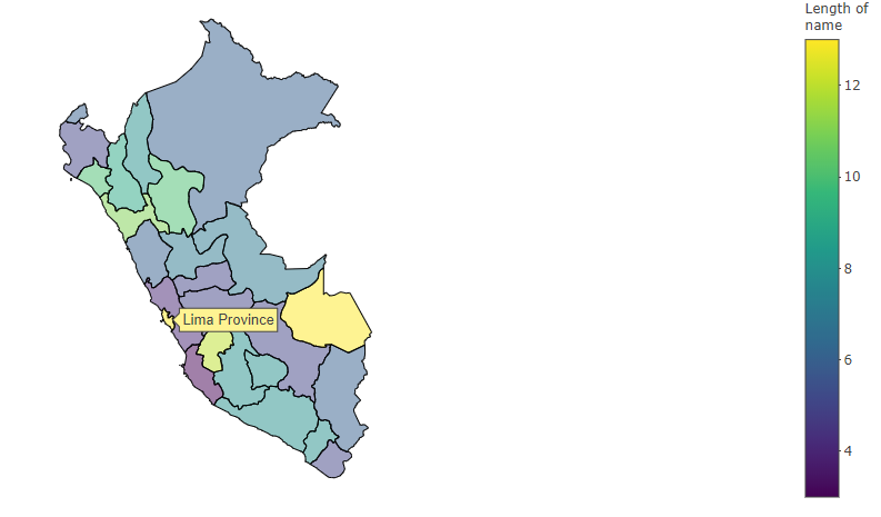
No tengo una respuesta exacta, en el archivo sf esa región es llamada Lima province, pero no he buscado la documentación para saber cuál es el criterio.

[Atalaveracuya]

He desagregado la base de datos deacuerdo al mapa. WeTransfer - Send Large Files & Share Photos Online - Up to 2GB Free

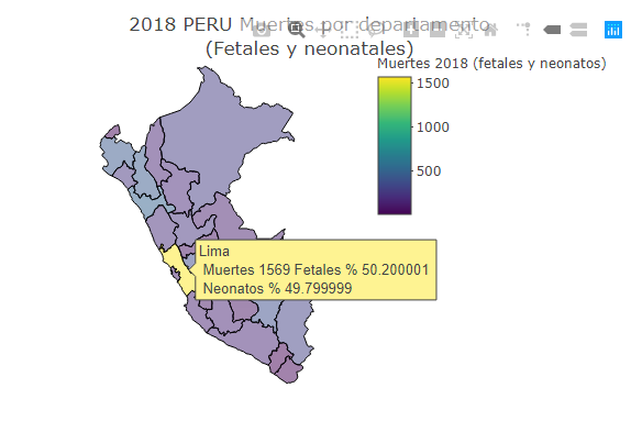
¿Cómo sería el gráfico?. Porque al parecer hay un error en la edición de las regiones del mapa. La región grande "Lima" (color amarillo) es la region "Lima provincias" y la más pequeña es la "Provincia de Lima", donde se encuentran los 43 distritos metropolitanos (Santiago de Surco, Chorrillos, San Borja, San Isidro, etc etc)

[andresrcs]

Ten en cuenta que las clasificaciones de regiones administrativas no son estándares a nivel internacional y que la fuente de estos mapas no es local (no lo he generado yo, solo lo he simplificado para que el renderizado sea más rápido), por ejemplo en esta otra fuente (un paquete R) el nombre "Lima Province" y los limites de la región son los mismos.

Nota: Si aún tienes más dudas sobre este tema, por favor continúa la conversación en Ingles, es el idioma oficial del foro y al usar español estás excluyendo a la gran mayoría de la conversación (lo que también disminuye tus probabilidades de obtener ayuda).

library(tidyverse)
library(rnaturalearth)

ne_states(country = "peru", returnclass = "sf") %>%
    select(name) %>% 
    filter(str_detect(name, "Lima"))
#> Simple feature collection with 2 features and 1 field
#> geometry type:  MULTIPOLYGON
#> dimension:      XY
#> bbox:           xmin: -77.8906 ymin: -13.32044 xmax: -75.4672 ymax: -10.28681
#> epsg (SRID):    4326
#> proj4string:    +proj=longlat +datum=WGS84 +no_defs
#>            name                       geometry
#> 1          Lima MULTIPOLYGON (((-76.24919 -...
#> 2 Lima Province MULTIPOLYGON (((-76.79908 -...

^{Created on 2019-09-07 by the reprex package (v0.3.0.9000)}

[Atalaveracuya]

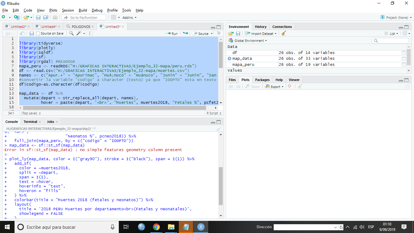
Use QGIS to generate my shapefile from the departments of Peru with the province of Lima and Callao (attached shapefile and database) I configured the database to join it to the shapefile, but when executing "sf :: st_sf (map_data) "I get the error: Error in sf :: st_sf (map_data): no simple features geometry column present

download shapefile and database: WeTransfer - Send Large Files & Share Photos Online - Up to 2GB Free

library(tidyverse)
library(plotly)
library(sqldf)
library(sf)
library(rgdal) #READ0GR
mapa_peru <- readRDS("H:/GRAFICAS INTERACTIVAS/Ejemplo_32-mapa/peru.rds")
df <- read.csv("H:/GRAFICAS INTERACTIVAS/Ejemplo_32-mapa/muertes.csv")
names <- c("Apur.+" = "Apurímac", "Huánuco" = "Huánuco", "Junin" = "Junín", "San Martin" = "San Martín")
#convertir la variable "codigo" a character (texto) ya que "IDDPTO" esta en texto 
df$codigo=as.character(df$codigo)

map_data <- df %>% 
  mutate(depart = str_replace_all(depart, names),
         hover = paste(depart, '<br>', "Muertes", muertes2018, "Fetales %", pcfet2018, "<br>",
                       "Neonatos %", pcneo2018)) %>% 
  full_join(mapa_peru, by = c("codigo" = "IDDPTO"))
map_data <- sf::st_sf(map_data)

plot_ly(map_data, color = I("gray90"), stroke = I("black"), span = I(1)) %>% 
  add_sf(
    color = ~muertes2018, 
    split = ~depart, 
    span = I(1),
    text = ~hover,
    hoverinfo = "text",
    hoveron = "fills"
  ) %>%
  colorbar(title = "Muertes 2018 (fetales y neonatos)") %>%
  layout(
    title = '2018 PERU Muertes por departamento<br>(Fetales y neonatales)',
    showlegend = FALSE
  )

[andresrcs]

@Atalaveracuya

Use QGIS to generate my shapefile

A Shape file (shp) is not the same as a Simple Features file (sf), you would have to convert it to a sf file first, like in this example.

library(tidyverse)
library(plotly)
library(sf)

mapa_peru <- read_sf("PERUFINAL.shp")
df <- read.csv("muertes.csv", stringsAsFactors = FALSE)
names <- c("Apur.+" = "Apurímac", "Huánuco" = "Huánuco", "Junin" = "Junín", "San Martin" = "San Martín")

map_data <- df %>% 
    mutate(depart = str_replace_all(depart, names),
           hover = paste(depart, "<br>Muertes:",
                         muertes2018,
                         "<br> Fetales:", scales::number(pcfet2018, suffix = " %", accuracy = 0.1),
                         "<br> Neonatos:", scales::number(pcneo2018, suffix = " %", accuracy = 0.1)
                         )
           ) %>% 
    full_join(mapa_peru, by = c("codigo" = "IDDPTO")) %>% 
    st_sf()

plot_ly(map_data, color = I("gray90"), stroke = I("black"), span = I(1)) %>% 
    add_sf(
        color = ~muertes2018, 
        split = ~depart, 
        span = I(1),
        text = ~hover,
        hoverinfo = "text",
        hoveron = "fills"
    ) %>%
    colorbar(title = "Número de<br>Muertes") %>%
    layout(
        title = 'Muertes Fetales y Neonatales por Departamento<br>Perú - 2018',
        showlegend = FALSE
    )

And, as a side comment, the extreme difference among Lima province and every other department is due to the difference in population density, I think you should consider using a transformation like number of deaths per 100 000 population