Create a common legend from multiple plots in a list

[jesse.f.lamb]

Hello,

Goal: To plot multiple fish diet taxa bar plots from multiple years w/ one common legend. I perform diet analysis of juvenile fish. It is common to plot the diet composition of fish diet data in terms of percent composition within a stomach by fish size. Here's an example from my paper from a couple years ago:

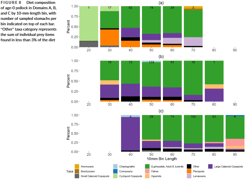
A, B, and C in this plot represent three different spatial regions where the fish were collected. For this I made three separate plots, created my own color palette for all prey taxa, then used "common.legend" in ggarrange:

s.a<-ggplot(data= Adb10, aes(x=Binn10, y=PreyPctTtl,fill=Taxa)) +
  geom_bar(stat = "identity", position = "fill")+ 
  annotate("text", x = An$Binn10, y = 1, label= (An$nCount), vjust = 1.1 ) # N of Fish per 10mmBin

  s.1.a <- s.a + labs(title="A") +
  labs( y="Percent") + #x="10mm Bin Length",
   scale_fill_manual(values = jColors) +  # jColors is the vector will all possible taxa colors
   scale_x_discrete(expand = c(0,0)) +
   scale_y_continuous(breaks = seq(0,1, by = .25), expand = c(0,0))
   
s.2.A <- s.1.a + theme(plot.title = element_text(hjust = 0.5)) + 
  theme(plot.title= element_text(size=(rel(1.4)))) +           
  #theme(axis.title.x = element_text(size=rel(1.25))) +  
  theme(axis.title.x = element_blank()) +
  theme(axis.title.y = element_text(size=rel(1.25))) +        
  theme(axis.text = element_text(size=rel(1.15)))+
  theme(panel.border = element_blank())+
  theme(panel.grid.major = element_blank())+
  theme(panel.background = element_blank(),
        panel.grid.major = element_blank(),
        panel.grid.minor = element_blank())

I copied and pasted this same code for regions 'B', and 'C', then:

P <- ggarrange(s.2.A,s.2.B,s.2.C, ncol=1,nrow=3,
  common.legend = TRUE, legend = "bottom")

Note that not all prey taxa are represented in every plot, yet all prey taxa are represented in the legend.

My next project is to do analysis of multiple years (n = 7 )of this same type of fish diet data, and would like to plot all seven years in one giant plot. There are 21 potential taxa over these 7 years, and not one year has all 21 prey taxa within it.

Here's an example of the data I'm plotting:

> head(Diet_Bar_Plot)
# A tibble: 6 × 5
# Groups:   Year, Binn10, Taxa [6]
  Taxa                          Year  Binn10 PreyPctTtl nCount
  <fct>                         <fct> <fct>       <dbl>  <int>
1 Large Calanoid Copepods       2003  40          90.2       1
2 Small Calanoid Copepods       2003  40           9.81      1
3 Euphausiids, Adult & Juvenile 2003  50          39.7      28
4 Large Calanoid Copepods       2003  50          22.7      28
5 Pteropods                     2003  50          12.3      28
6 Small Calanoid Copepods       2003  50          11.6      28

Where Binn10 = size of fish (mm), PreyPctTtl = percent taxa found in fish at that bin size, and nCount = how many fish of that bin size were analyzed.

I then created a function for all my bar plots, pretty much exactly the same as above:

DietBarF <- function(z,zz){ggplot(data= z, aes(x=Binn10, y=PreyPctTtl,fill=Taxa)) +
  geom_bar(stat = "identity", position = "fill")+ 
  annotate("text", x = z$Binn10, y = 1, label= (z$nCount), vjust = 1.1 ) + # N of Fish per 10mmBin
     labs(title= zz) +
  labs( y="Percent") + #x="10mm Bin Length",
   scale_fill_manual(values = jColors) +  # jcolors is the vector of assigned taxa colors
   scale_x_discrete(expand = c(0,0)) +
   scale_y_continuous(breaks = seq(0,1, by = .25), expand = c(0,0)) +
    theme(plot.title = element_text(hjust = 0.5)) + 
    theme(plot.title= element_text(size=(rel(1.4)))) +           
   theme(axis.title.x = element_text(size=rel(1.25))) +  
   theme(axis.title.x = element_blank()) +
   theme(axis.title.y = element_text(size=rel(1.25))) +        
   theme(axis.text = element_text(size=rel(1.15)))+
   theme(panel.border = element_blank())+
   theme(panel.grid.major = element_blank())+
   theme(panel.background = element_blank(),
         panel.grid.major = element_blank(),
         panel.grid.minor = element_blank())}

then I create plots for all years using purrr::map2. I then plot using ggarrange:

Diet_Bar_Plots <- Diet_Bar_Plot   %>%  dplyr::group_by(Year) %>% 
  tidyr::nest() %>% ungroup() %>%  mutate(plot = purrr::map2(data,Year,DietBarF))

All_Diet_Plots <- Diet_Bar_Plots$plot

ggarrange(plotlist = All_Diet_Plots, ncol = 2, nrow = 5,
          common.legend = TRUE, legend = "right")

Here's how it looks like (remember, it's preliminary):

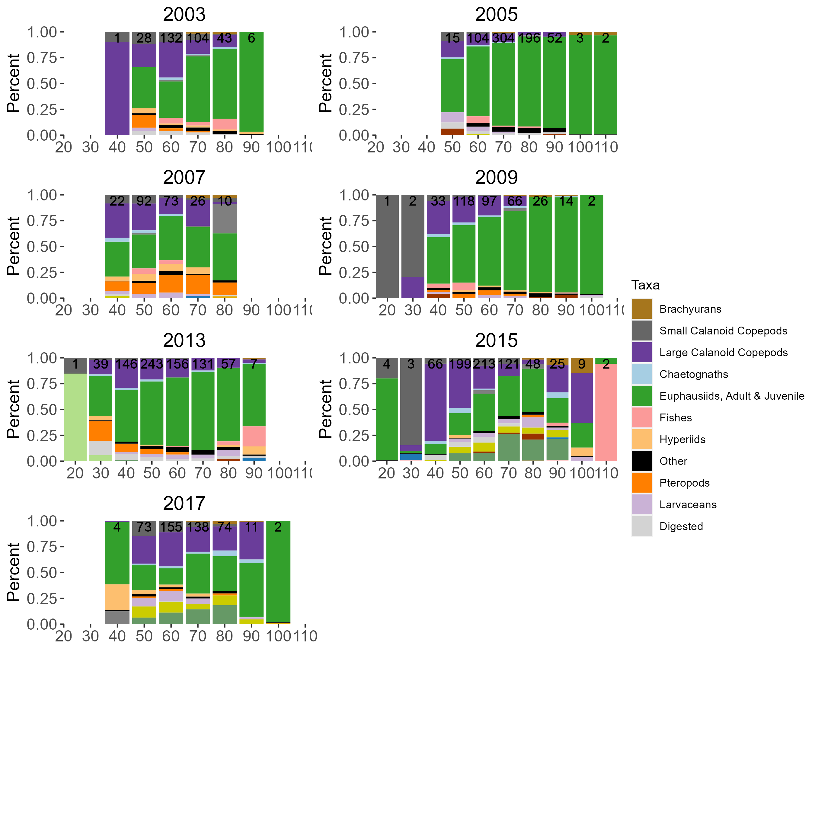
There are only 11 of the possible 21 taxa represented in the legend. I have also tried using 'legend_grob' and I keep getting the same 11 taxa. I'm guessing it's only taking the taxa from 2003, the first plot:

gL <- get_legend(All_Diet_Plots)
ggarrange(plotlist = All_Diet_Plots, ncol = 2, nrow = 5,
          common.legend = TRUE, legend = "right", legend.grob = gL)

In the end, I believe my question is how to combine all possible prey taxa from my plot list from above and create one legend?

Thank you for your time.

[nirgrahamuk]

the solution, is that the for the first plot being ggarranged with common.legend option; have that plot generate a complete legend with all the required levels by using drop=FALSE argument in the scale_fill_manual you are runing on it.

for example

   scale_fill_manual(values = jColors) +  

becomes

   scale_fill_manual(values = jColors, drop=FALSE) +

[jesse.f.lamb]

That works! Thank you for your help.