Common axis title in grid.arrange

[Gabbi]

Hello,
I need to format the common axis title in grid.arrange.
Here is an example:

plots

p1 <- ggplot(data = mtcars, aes(x = mpg, y = cyl))
p2 <- ggplot(data = mtcars, aes(x = mpg, y = cyl))
p3 <- ggplot(data = mtcars, aes(x = mpg, y = cyl))
p4 <- ggplot(data = mtcars, aes(x = mpg, y = cyl))

General axis labels

yleft <- textGrob("name 1 (tha^-1)", rot = 90, gp = gpar(fontsize = 20))
yright <- textGrob("name 2 and 3 (t ha^-1)", rot = 270, gp = gpar(fontsize = 20))
bottom <- textGrob("age (years)", gp = gpar(fontsize = 20))

Join plots

uni <- grid.arrange(p1, p2, p3, p4, ncol = 2, nrow = 2, right = yright, left = yleft, bottom = bottom)

How can I format the superscripts characters and use different colors by word (like ggtext package does)?
I've tried several ways to do it and it still didn't work.
Can someone help?

[joels]

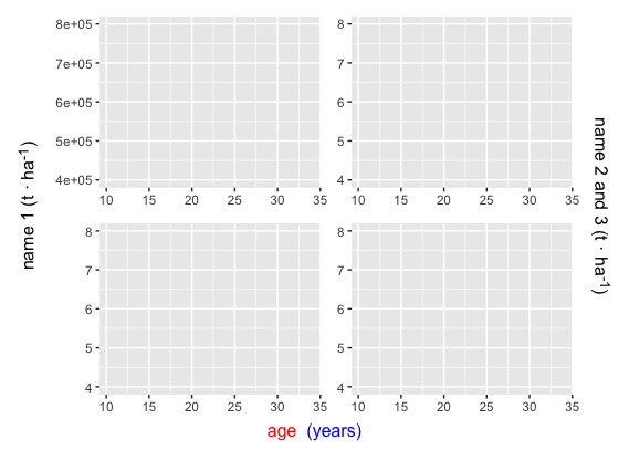
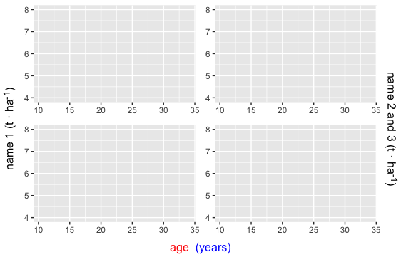
For the superscripts and subscripts you can use plotmath expressions (see ?plotmath), but gridtext is easier, since we can use markdown syntax (or html, if needed) for text formatting. Here are both approaches. The rendered version uses gridtext.

library(tidyverse)
library(gridExtra)
library(grid)
library(gridtext)

p1 <- ggplot(data = mtcars, aes(x = mpg, y = cyl)) 
p2 <- ggplot(data = mtcars, aes(x = mpg, y = cyl))
p3 <- ggplot(data = mtcars, aes(x = mpg, y = cyl))
p4 <- ggplot(data = mtcars, aes(x = mpg, y = cyl))

# Remove axis titles from all plots
p = list(p1,p2,p3,p4) %>% map(~.x + labs(x=NULL, y=NULL))

# plotmath expressions
yleft <- textGrob(expression(paste("name 1 (t"%.%"ha"^"-1"*")")), 
                  rot = 90, gp = gpar(fontsize = 20))
yright <- textGrob(expression(paste("name 2 and 3 (t"%.%"ha"^"-1"*")")), 
                   rot = 270, gp = gpar(fontsize = 20))

bottom <- textGrob("age (years)", gp = gpar(fontsize = 20, col="red"))

# gridtext
yleft = richtext_grob("name 1 (t &middot; ha^(-1))", rot=90)

yright = richtext_grob("name 2 and 3 (t &middot; ha^(-1))", rot=-90)

bottom = richtext_grob(
  text = '<span style="color:red">age</span> <span style="color:blue">(years)</span>'
)

# Lay out plots
uni <- grid.arrange(grobs=p, ncol = 2, nrow = 2, 
                    right = yright, left = yleft, bottom = bottom)

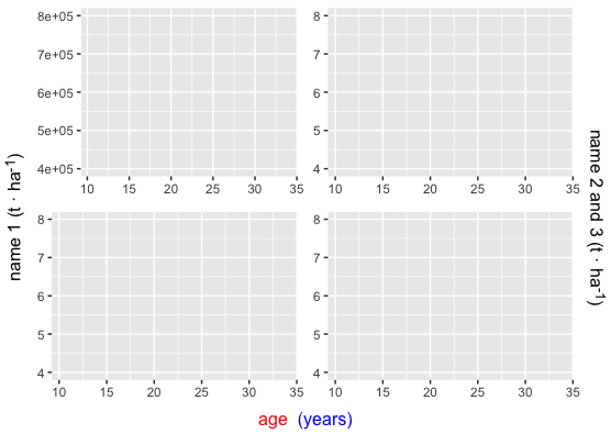
Note that If the axis labels have different widths, grid.arrange won't line up the panels. For example:

p[[1]] <- ggplot(data = mtcars %>% mutate(cyl=cyl*1e5), 
             aes(x = mpg, y = cyl)) 

#Join plots
uni <- grid.arrange(grobs=p, ncol = 2, nrow = 2, 
                    right = yright, left = yleft, bottom = bottom)

The patchwork package is another option for laying out multiple plots and it also lines up the plot panels. Unfortunately, patchwork doesn't provide an easy way to add spanning axis titles (like the bottom, left, and right arguments of grid.arrange) so we have to manually set the widths for those grobs, relative to the plot grobs.

library(patchwork)

{ wrap_elements(yleft) + 
    {{p[[1]] + p[[2]]} / {p[[3]] + p[[4]]}}  + 
    wrap_elements(yright) +
    plot_layout(widths=c(1,20,1)) } / 
  bottom + 
  plot_layout(heights=c(100,1))

[Gabbi]

It worked perfectly!! Thank you very much!!