combine plot using ggplot and a dataframe

mslider · August 23, 2023, 9:10am

--Hi all,

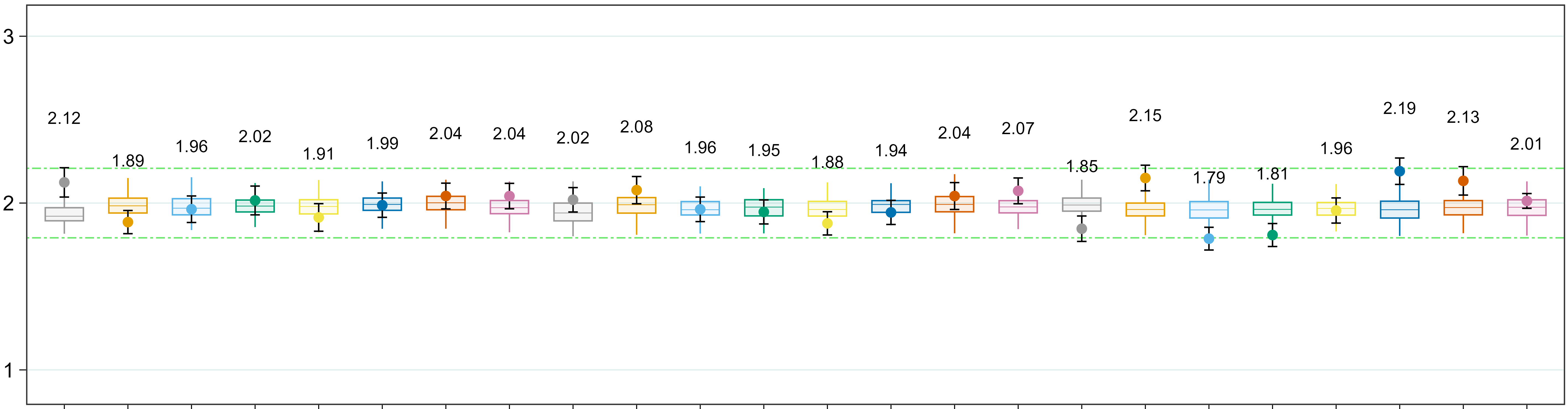
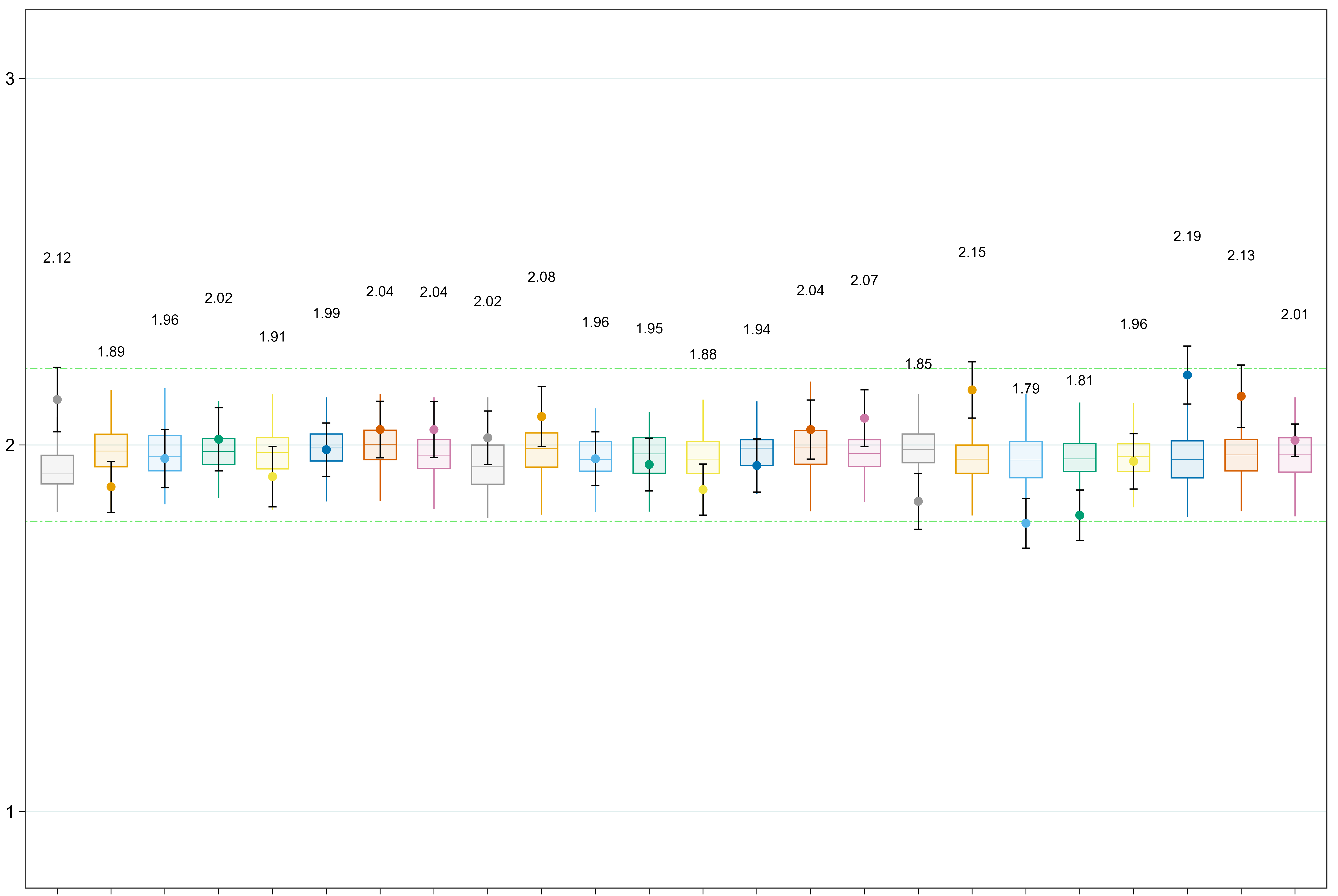
i try to use ggplot to make a graph with 2 plots: a boxplot with errorbar and add point on it.
When i disable boxplot (geom_boxplot) and errorbar (stat_boxplot) it works but i try to add boxplot it failed with:

Error in geom_boxplot():
! Problem while computing aesthetics.
i Error occurred in the 3rd layer.
Caused by error in check_aesthetics():
! Aesthetics must be either length 1 or the same as the data (6864)
x Fix the following mappings: label.
I don't find a solution, if you have an idea to handle this problem . Thank you .

ggplot(all_df) + aes(x=id, y=median, col=id, label=mean +
    geom_text(size = 2.6, nudge_y = df$sd+0.3, color="black", family="Roboto Condensed") +
    scale_x_discrete(limits=chr)+ labs(y ="blabla", x=" ") + scale_y_continuous(expand = c(0,0),breaks = c(1:5)) + coord_cartesian(ylim = c(-0.15, 5)) +
    geom_point(size=3) +
    geom_boxplot(data=reshape2::melt(all_df[,c(1,5:ncol(all_df))]), aes(x = id,y = value),width = 0.6, fill = "white", outlier.shape=NA, position="identity", alpha=.5) +
    stat_boxplot(data=reshape2::melt(all_df[,c(1,5:ncol(all_df))]), aes(x = id,y = value),geom ='errorbar', width = 0.3, color="darkred") +
    theme_bw() +
      theme(
           legend.position="none",
           plot.title = element_text(color="#00A4C4", size=11, face="bold", family="Helvetica"),
           axis.title.y = element_text(vjust = 0.5, margin = margin(t = 0, r = 10, b = 0, l = 0),color="black", size=11, face="bold", family="Roboto Condensed"),
           panel.grid.major.y= element_line(color="azure2",size = 0.25, linetype = 'solid'),
           panel.grid.minor.y=element_blank(),
           panel.grid.major.x=element_blank(),
           panel.grid.minor.x=element_blank(),
           panel.background = element_rect(fill = "white", colour="black", size = 0.5, linetype = "solid"),
           axis.text.x = element_text(face="plain", color="black", size = 9, family="Roboto Condensed"),
           axis.text.y = element_text(face="plain", color="black", size = 9, family="Roboto Condensed"),
           axis.line = element_line(colour = "black", size = 0, linetype = "solid"),
           axis.ticks = element_line(color = "black", size = 0.2),
           axis.ticks.length = unit(3,"pt"),
           plot.caption = element_text(color="black", size=8, family="Roboto Condensed")
          )
          

dataframe:

id	median	sd	mean	V1	V2	V3	V4	V5	V6	V7	V8	V9	V10	V11	V12	V13	V14	V15	V16	V17	V18	V19	V20	V21	V22	V23	V24	V25	V26	V27	V28
id_1	2.128834	0.08789907	2.13	NA	NA	NA	NA	NA	NA	NA	NA	NA	NA	NA	NA	NA	NA	NA	NA	NA	NA	NA	NA	NA	NA	NA	NA	NA	NA	NA	NA
id_2	1.886293	0.06952459	1.89	1.943574	2.008329	1.93	1.854861	1.95	2.065349	1.943712	1.85	1.854861	1.89	1.92	1.9	1.904362	NA	2.043071	1.89	1.89	1.99	1.989738	1.989738	NA	NA	NA	NA	NA	NA	NA	NA
id_3	1.963582	0.0794687	1.96	1.941002	2.00696	1.89	1.913491	2.05	1.973865	2.074511	1.91	1.913491	2.03	1.92	1.91	1.909287	NA	2.035436	2.05	2.05	1.88	1.876261	1.876261	1.94	NA	1.94	1.938657	1.938657	1.938657	1.94	NA
id_4	2.015077	0.08624216	2.02	1.968469	1.826555	1.91	1.986253	2.08	1.898847	1.952565	1.99	1.986253	1.95	1.97	2.01	2.005393	NA	1.939542	1.97	1.97	1.92	1.917922	1.917922	2.07	NA	2.07	2.065553	2.065553	2.065553	2.07	NA
id_5	1.914766	0.08259576	1.91	1.834312	1.802306	1.9	1.986253	2.02	1.962442	1.955721	1.99	1.986253	1.93	1.98	2.11	2.112612	NA	1.943656	2.02	2.02	2.05	2.046592	2.046592	2.18	NA	2.18	2.183175	2.183175	2.183175	2.18	NA
id_6	1.986747	0.07278337	1.99	2.001663	1.943493	2.13	2.041936	1.99	1.993138	1.883518	2.04	2.041936	2.09	1.99	2.1	2.101173	NA	2.045536	2.01	2.01	1.99	1.991448	1.991448	2.04	NA	2.04	2.042928	2.042928	2.042928	2.04	NA
id_7	2.041665	0.07714729	2.04	1.859711	1.859711	1.98	2.105747	2	2.056169	1.900714	2.11	2.105747	1.98	2.01	2.03	2.02628	NA	2.120911	1.92	1.92	2.05	2.051777	2.051777	1.97	NA	1.97	1.966943	1.966943	1.966943	1.97	NA
id_8	2.042482	0.07622628	2.04	1.812517	1.859711	1.88	2	1.97	1.922302	1.95275	2	2	1.96	2.02	2.08	2.078984	NA	2.083413	1.95	1.95	2.06	2.060142	2.060142	2.01	NA	2.01	2.0149	2.0149	2.0149	2.01	NA
id_9	2.016395	0.07308968	2.02	1.978693	1.996633	1.96	1.829928	2.03	1.893179	1.903842	1.83	1.829928	1.97	1.86	1.84	1.843262	NA	1.936815	2.02	2.02	1.93	1.931962	1.931962	2	NA	2	2.003325	2.003325	2.003325	2	NA
id_10	2.077008	0.0815966	2.08	1.996633	1.978693	1.91	1.962029	2	1.980806	1.924015	1.96	1.962029	1.87	1.81	1.84	1.844572	NA	1.968375	2.05	2.05	1.95	1.947814	1.947814	1.98	NA	1.98	1.975084	1.975084	1.975084	1.98	NA
id_11	1.961878	0.07351241	1.96	1.972671	1.97019	1.94	2.070531	2.02	2.025465	2.156081	2.07	2.070531	1.96	2.1	1.98	1.976377	NA	2.081182	2.04	2.04	2.1	2.096287	2.096287	1.93	NA	1.93	1.926265	1.926265	1.926265	1.93	NA
id_12	1.945766	0.07195502	1.95	1.955244	NA	1.87	2.035077	1.95	1.963235	1.894812	2.04	2.035077	2	1.88	2.02	2.021599	NA	1.938052	2.02	2.02	2.05	2.052677	2.052677	2.05	NA	2.05	2.054805	2.054805	2.054805	2.05	NA
id_13	1.879229	0.06970549	1.88	1.959484	1.958237	2.05	1.864796	2.09	1.97812	1.914872	1.86	1.864796	1.97	2.07	1.95	1.953903	NA	2.040437	2.01	2.01	1.99	1.985977	1.985977	1.85	NA	1.85	1.84931	1.84931	1.84931	1.85	NA
id_14	1.94496	0.0723412	1.94	NA	NA	NA	NA	NA	NA	NA	NA	NA	NA	NA	NA	NA	NA	NA	NA	NA	NA	NA	NA	NA	NA	NA	NA	NA	NA	NA	NA
id_15	2.041629	0.08052228	2.04	1.924443	1.922322	1.92	2.038979	2.05	1.961567	1.909779	2.04	2.038979	2.04	2.1	2.01	2.005397	NA	1.97519	2.04	2.04	NA	NA	NA	2.06	NA	2.06	2.059796	2.059796	2.059796	2.06	NA
id_16	2.074961	0.07732924	2.07	1.859711	1.812517	1.85	2.004453	1.94	1.918225	1.900714	2	2.004453	1.86	1.93	2.01	2.014328	NA	1.935574	2.01	2.01	1.91	1.908511	1.908511	NA	NA	NA	NA	NA	NA	NA	NA
id_17	1.845441	0.07625053	1.85	1.849481	1.855857	2.03	1.963576	2	2.1258	1.862597	1.96	1.963576	1.97	1.96	1.98	1.978153	NA	2.122136	1.96	1.96	2.05	2.046269	2.046269	2.14	NA	2.14	2.138137	2.138137	2.138137	2.14	NA
id_18	2.148845	0.07670523	2.15	NA	NA	NA	NA	NA	NA	NA	NA	NA	NA	NA	NA	NA	NA	NA	NA	NA	NA	NA	NA	NA	NA	NA	NA	NA	NA	NA	NA
id_19	1.785136	0.06809043	1.79	1.846748	1.846748	1.96	2.025214	2	2.040753	1.944469	2.03	2.025214	2.02	2.02	1.98	1.976928	NA	2.161579	1.96	1.96	2.11	2.107394	2.107394	1.94	NA	1.94	1.941796	1.941796	1.941796	1.94	NA
id_20	1.807889	0.06885714	1.81	2.019918	1.832117	1.96	1.972668	2.04	2.007485	2.025464	1.97	1.972668	1.94	2.05	1.94	1.938214	NA	1.884127	1.94	1.94	2	1.998316	1.998316	1.98	NA	1.98	1.982616	1.982616	1.982616	1.98	NA
id_21	1.954877	0.07543282	1.95	NA	1.95418	NA	1.917188	1.97	2.016743	1.856908	1.92	1.917188	2.02	1.95	2	2.003238	NA	1.965553	1.92	1.92	2.02	2.023391	2.023391	1.96	NA	1.96	1.956948	1.956948	1.956948	1.96	NA
id_22	2.190368	0.079101	2.19	1.854569	1.85571	2.02	1.966078	1.94	1.967194	1.959532	1.97	1.966078	2.01	1.96	1.91	1.90588	NA	1.962941	2.02	2.02	1.85	1.846493	1.846493	2.02	NA	2.02	2.022455	2.022455	2.022455	2.02	NA
id_23	2.132497	0.08516972	2.13	2.00696	1.941002	2	2.012601	2.13	2.039295	1.918657	2.01	2.012601	2.05	2.01	1.84	1.841972	NA	2.093189	1.93	1.93	1.97	1.973266	1.973266	2	NA	2	1.996848	1.996848	1.996848	2	NA
id_24	2.013253	0.04435878	2.01	1.957032	1.957011	2.03	2.026913	1.99	1.931749	1.956258	2.03	2.026913	2.02	2	2.08	2.08422	NA	1.888023	2.08	2.08	1.92	1.919167	1.919167	2.04	NA	2.04	2.044944	2.044944	2.044944	2.04	NA

FJCC · August 23, 2023, 2:56pm

The following code does not throw an error. I removed the call to scale_x_discrete() because there is no object named chr. Your original code lacked a closing parenthesis on the first aes() . In geom_text(), you referred to df$sd but there is no data frame named df, so I changed that to all_df$sd. I moved the use of reshape::melt outside of the plotting code to make it more readable.

DF2 <- reshape2::melt(all_df[,c(1,5:ncol(all_df))])
ggplot() + 
  geom_text(data = all_df,mapping = aes(x=id, y=median, col=id, label=mean),
            size = 2.6, nudge_y = all_df$sd+0.3, color="black", family="Roboto Condensed") + #scale_x_discrete(limits=chr)+
  labs(y ="blabla", x=" ") + scale_y_continuous(expand = c(0,0),breaks = c(1:5)) + coord_cartesian(ylim = c(-0.15, 5)) +
  geom_point(data = all_df,mapping = aes(x=id, y=median, col=id, label=mean), size=3) +
  geom_boxplot(data=DF2, mapping = aes(x = id,y = value),width = 0.6, fill = "white", outlier.shape=NA, position="identity", alpha=.5) +
  stat_boxplot(data=DF2, aes(x = id,y = value),geom ='errorbar', width = 0.3, color="darkred") +
  theme_bw() +
  theme(
    legend.position="none",
    plot.title = element_text(color="#00A4C4", size=11, face="bold", family="Helvetica"),
    axis.title.y = element_text(vjust = 0.5, margin = margin(t = 0, r = 10, b = 0, l = 0),color="black", size=11, face="bold", family="Roboto Condensed"),
    panel.grid.major.y= element_line(color="azure2",size = 0.25, linetype = 'solid'),
    panel.grid.minor.y=element_blank(),
    panel.grid.major.x=element_blank(),
    panel.grid.minor.x=element_blank(),
    panel.background = element_rect(fill = "white", colour="black", size = 0.5, linetype = "solid"),
    axis.text.x = element_text(face="plain", color="black", size = 9, family="Roboto Condensed"),
    axis.text.y = element_text(face="plain", color="black", size = 9, family="Roboto Condensed"),
    axis.line = element_line(colour = "black", size = 0, linetype = "solid"),
    axis.ticks = element_line(color = "black", size = 0.2),
    axis.ticks.length = unit(3,"pt"),
    plot.caption = element_text(color="black", size=8, family="Roboto Condensed")
  )

mslider · August 24, 2023, 4:30pm

hi,

i have updated my code with your remarks and yes it works fine now.
I have just a question regarding scale: is it possible to use different scales: one for the boxplot (DF2 dataframe) and other for geom_point (all_df dataframe).
I say that because the boxplot looks squashed when i use ggsave such as: ggsave(plot =myplot, filename = 'boxplot.png', dpi=600, dev='png', width = 25, height = 8, units = "cm")

thank you --

FJCC · August 24, 2023, 5:15pm

If you want to have a second y axis, you can use code like the following. Notice that in geom_boxplot() and stat_boxplot() I double the value of the plotted points and in the sec_axis() function, I divide the displayed labels by a factor of two. The box plots are plotted against the axis on the left, but the labels on the right show the original y values.

ggplot() + 
  geom_text(data = all_df,mapping = aes(x=id, y=median, col=id, label=mean),
            size = 2.6, nudge_y = all_df$sd+0.3, color="black", family="Roboto Condensed") + #scale_x_discrete(limits=chr)+
  labs(y ="blabla", x=" ") + 
  scale_y_continuous(expand = c(0,0),breaks = c(1:5), sec.axis = sec_axis(~ . / 2, name = "box plots")) + 
  coord_cartesian(ylim = c(-0.15, 5)) +
  geom_point(data = all_df,mapping = aes(x=id, y=median, col=id, label=mean), size=3) +
  geom_boxplot(data=DF2, mapping = aes(x = id,y = value * 2),width = 0.6, fill = "white", outlier.shape=NA, position="identity", alpha=.5) +
  stat_boxplot(data=DF2, aes(x = id,y = value * 2),geom ='errorbar', width = 0.3, color="darkred") +
  theme_bw() +
  theme(
    legend.position="none",
    plot.title = element_text(color="#00A4C4", size=11, face="bold", family="Helvetica"),
    axis.title.y = element_text(vjust = 0.5, margin = margin(t = 0, r = 10, b = 0, l = 0),color="black", size=11, face="bold", family="Roboto Condensed"),
    panel.grid.major.y= element_line(color="azure2",size = 0.25, linetype = 'solid'),
    panel.grid.minor.y=element_blank(),
    panel.grid.major.x=element_blank(),
    panel.grid.minor.x=element_blank(),
    panel.background = element_rect(fill = "white", colour="black", size = 0.5, linetype = "solid"),
    axis.text.x = element_text(face="plain", color="black", size = 9, family="Roboto Condensed"),
    axis.text.y = element_text(face="plain", color="black", size = 9, family="Roboto Condensed"),
    axis.line = element_line(colour = "black", size = 0, linetype = "solid"),
    axis.ticks = element_line(color = "black", size = 0.2),
    axis.ticks.length = unit(3,"pt"),
    plot.caption = element_text(color="black", size=8, family="Roboto Condensed")
  )

mslider · August 25, 2023, 2:54pm

we misunderstood each other, that's not what I meant.

when i use this command to save the image: ggsave(plot = gg, filename = 'boxplot_test_1.png', dpi=600, dev='png', width = 25, height = 8, units = "cm")
the boxplot appears compressed (see attachment),
whereas when i use ggsave(plot = gg, filename = 'boxplot_test_1.png', dpi=600, dev='png', width = 25, units = "cm") the box plot is longer and more normal (see attachment)

FJCC · August 25, 2023, 3:36pm

I think all of the difference in the two plots is accounted for by the difference in the setting of the height argument in ggsave(). In the second call to ggsave(), you don't set height and it defaults to a value that you happen to prefer.

ggsave(plot = gg, filename = 'boxplot_test_1.png', dpi=600, dev='png', 
       width = 25, height = 8, units = "cm")

ggsave(plot = gg, filename = 'boxplot_test_1.png', dpi=600, dev='png', 
       width = 25, units = "cm")

system · October 6, 2023, 3:37pm

This topic was automatically closed 42 days after the last reply. New replies are no longer allowed.

If you have a query related to it or one of the replies, start a new topic and refer back with a link.