Hi there,
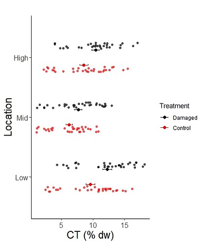
I produced a dot plot on 6 different treatments (trees under 6 different conditions; in column " Location.Treatment " in my raw data). For each of these “ Location.treatment” categories, I calculated a mean value and the SE for a specific compound (%CT).
I am able to produce a plot where all the 6 treatments (in column " Location.Treatment") are separated (see code and Fig in red&black) so that each of two "con" and "exp" treatments (in the column "treatment") are nested within one of the three locations (High, mid, low; in the column "Location") (see plot that the code produces). This is the plot structure I want.
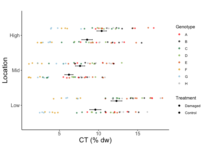
Now I would like to assign colors to the raw data points ( the “point cloud” next to each mean +SE value). Each of these points stems from a different "Genotype" and I would like to color code the points with regard to the genotypes (e.g. all points from Genotype A should be green, all points from Genotype B should be red etc.) I would like to use my own specified colors in the code (not the standard palette).
I tried did the following (without success)
- I added “aes(color=Genotype,….” into “geom_point(….)”
- I added my specific colors to “scale_color_manual”
scale_color_manual(labels=c("Control","Damaged"),values=c("red","black","#067c43","#89b651","#dc5b09","#e4a710","#92c5de","grey","#1d71b4","#7873a3"......
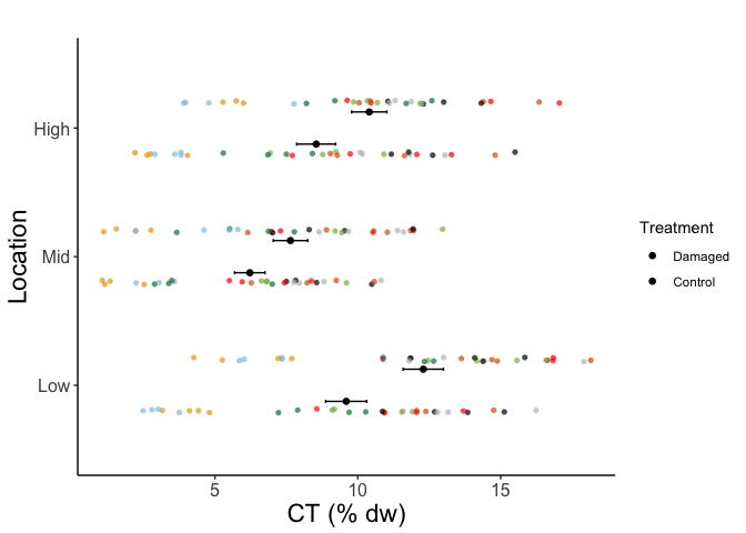
However, if I do that my “nested” plot structure disappears (i.e. I cannot visually differentiate between “con” and “exp” treatments nested within mid /high/)
Basically, all I want is to produce a plot that looks like the one in the red&black Figure but where the individual data points are colored according to “Genotypes”
Below is my code, relevant figures and my raw data.
Help is very much appreciated!
# CODE
require(ggplot2)

#REMOVE START FOR ANALYSIS
dta<-subset(dta_complete,Time=="Stop")
dta

#Calculation of SE
data_summary <- function(x) {
  m <- mean(x)
  ymin <- m-sd(x)/sqrt(length(x))
  ymax <- m+sd(x)/sqrt(length(x))
  return(c(y=m,ymin=ymin,ymax=ymax))
}

pd1 = position_dodge(0.5)

plot_CT<- ggplot(dta, aes(x=Location, y=CT, colour=Treatment,shape=Treatment)) +
  stat_summary(fun.data=data_summary, position=pd1, geom="errorbar", width=0.05) +
  stat_summary(fun.data=data_summary, position=pd1, geom="point", size=2) +
  geom_point(position=position_jitterdodge(dodge.width=0.8, jitter.height=0, jitter.width=0.2),
             alpha=0.7) +
  labs(title="", x="", y = "CT (% dw)")+
  scale_color_manual(labels=c("Control", "Damaged"),values=c("red","black"),guide = guide_legend(reverse = TRUE) )+
  scale_shape_manual(labels=c("Control", "Damaged"),name="Treatment",values = c(16,16),guide = guide_legend(reverse = TRUE) )+
  #Style of background
  theme_classic()+
  #Change title
  theme(plot.title = element_text(color="black", size=17, face="bold"))+
  #Font size axis
  theme(axis.text=element_text(size=12),
        axis.title=element_text(size=17))+
  scale_x_discrete("Location",labels = c("Low", "Mid", "High"),expand=c(0.1, 0.5))+
  coord_flip()

plot_CT
#CODE END
#RAW DATA

structure(list(Location = structure(c(2L, 3L, 1L, 2L, 3L, 1L,
2L, 3L, 1L, 2L, 3L, 1L, 2L, 1L, 2L, 3L, 1L, 2L, 3L, 1L, 2L, 3L,
1L, 2L, 3L, 1L, 2L, 3L, 1L, 2L, 3L, 1L, 2L, 3L, 1L, 2L, 3L, 1L,
2L, 3L, 1L, 2L, 3L, 1L, 2L, 3L, 1L, 2L, 3L, 1L, 2L, 3L, 1L, 2L,
3L, 1L, 2L, 3L, 1L, 2L, 3L, 1L, 2L, 3L, 1L, 2L, 3L, 1L, 2L, 3L,
1L, 2L, 3L, 1L, 2L, 3L, 1L, 2L, 3L, 1L, 2L, 3L, 1L, 2L, 3L, 1L,
3L, 1L, 2L, 3L, 1L, 2L, 3L, 1L, 2L, 3L, 1L, 2L, 3L, 1L, 2L, 3L,
1L, 2L, 3L, 1L, 2L, 3L, 1L, 2L, 3L, 1L, 2L, 3L, 1L, 2L, 3L, 1L,
2L, 3L, 1L, 2L, 3L, 1L, 2L, 3L, 1L, 2L, 3L, 1L, 2L, 3L, 1L, 2L,
3L, 1L, 2L, 3L, 1L, 2L, 3L, 1L, 2L, 3L, 1L, 2L, 3L, 1L, 2L, 3L,
1L, 2L, 3L, 1L, 2L, 3L, 1L, 2L, 3L, 1L, 2L, 3L, 1L, 2L, 3L, 1L,
2L, 3L, 1L, 2L, 3L, 1L, 2L, 3L, 1L, 2L, 3L, 1L, 2L, 3L, 1L, 2L,
3L, 1L, 2L, 3L, 1L, 2L, 3L, 1L), .Label = c("High", "Low", "Mid"
), class = "factor"), Treatment = structure(c(2L, 2L, 2L, 1L,
1L, 1L, 2L, 2L, 2L, 1L, 1L, 1L, 2L, 2L, 1L, 1L, 1L, 2L, 2L, 2L,
1L, 1L, 1L, 2L, 2L, 2L, 1L, 1L, 1L, 2L, 2L, 2L, 1L, 1L, 1L, 2L,
2L, 2L, 1L, 1L, 1L, 2L, 2L, 2L, 1L, 1L, 1L, 2L, 2L, 2L, 1L, 1L,
1L, 2L, 2L, 2L, 1L, 1L, 1L, 2L, 2L, 2L, 1L, 1L, 1L, 2L, 2L, 2L,
1L, 1L, 1L, 2L, 2L, 2L, 1L, 1L, 1L, 2L, 2L, 2L, 1L, 1L, 1L, 2L,
2L, 2L, 1L, 1L, 2L, 2L, 2L, 1L, 1L, 1L, 2L, 2L, 2L, 1L, 1L, 1L,
2L, 2L, 2L, 1L, 1L, 1L, 2L, 2L, 2L, 1L, 1L, 1L, 2L, 2L, 2L, 1L,
1L, 1L, 2L, 2L, 2L, 1L, 1L, 1L, 2L, 2L, 2L, 1L, 1L, 1L, 2L, 2L,
2L, 1L, 1L, 1L, 2L, 2L, 2L, 1L, 1L, 1L, 2L, 2L, 2L, 1L, 1L, 1L,
2L, 2L, 2L, 1L, 1L, 1L, 2L, 2L, 2L, 1L, 1L, 1L, 2L, 2L, 2L, 1L,
1L, 1L, 2L, 2L, 2L, 1L, 1L, 1L, 2L, 2L, 2L, 1L, 1L, 1L, 2L, 2L,
2L, 1L, 1L, 1L, 2L, 2L, 2L, 1L, 1L, 1L), .Label = c("Con", "Exp"
), class = "factor"), Time = structure(c(2L, 2L, 2L, 2L, 2L,
2L, 2L, 2L, 2L, 2L, 2L, 2L, 2L, 2L, 2L, 2L, 2L, 2L, 2L, 2L, 2L,
2L, 2L, 2L, 2L, 2L, 2L, 2L, 2L, 2L, 2L, 2L, 2L, 2L, 2L, 2L, 2L,
2L, 2L, 2L, 2L, 2L, 2L, 2L, 2L, 2L, 2L, 2L, 2L, 2L, 2L, 2L, 2L,
2L, 2L, 2L, 2L, 2L, 2L, 2L, 2L, 2L, 2L, 2L, 2L, 2L, 2L, 2L, 2L,
2L, 2L, 2L, 2L, 2L, 2L, 2L, 2L, 2L, 2L, 2L, 2L, 2L, 2L, 2L, 2L,
2L, 2L, 2L, 2L, 2L, 2L, 2L, 2L, 2L, 2L, 2L, 2L, 2L, 2L, 2L, 2L,
2L, 2L, 2L, 2L, 2L, 2L, 2L, 2L, 2L, 2L, 2L, 2L, 2L, 2L, 2L, 2L,
2L, 2L, 2L, 2L, 2L, 2L, 2L, 2L, 2L, 2L, 2L, 2L, 2L, 2L, 2L, 2L,
2L, 2L, 2L, 2L, 2L, 2L, 2L, 2L, 2L, 2L, 2L, 2L, 2L, 2L, 2L, 2L,
2L, 2L, 2L, 2L, 2L, 2L, 2L, 2L, 2L, 2L, 2L, 2L, 2L, 2L, 2L, 2L,
2L, 2L, 2L, 2L, 2L, 2L, 2L, 2L, 2L, 2L, 2L, 2L, 2L, 2L, 2L, 2L,
2L, 2L, 2L, 2L, 2L, 2L, 2L, 2L, 2L), .Label = c("Start", "Stop"
), class = "factor"), Genotype = structure(c(7L, 7L, 7L, 7L,
7L, 7L, 4L, 4L, 4L, 4L, 4L, 4L, 6L, 6L, 6L, 6L, 6L, 2L, 2L, 2L,
2L, 2L, 2L, 3L, 3L, 3L, 3L, 3L, 3L, 8L, 8L, 8L, 8L, 8L, 8L, 1L,
1L, 1L, 1L, 1L, 1L, 5L, 5L, 5L, 5L, 5L, 5L, 4L, 4L, 4L, 4L, 4L,
4L, 3L, 3L, 3L, 3L, 3L, 3L, 2L, 2L, 2L, 2L, 2L, 2L, 6L, 6L, 6L,
6L, 6L, 6L, 8L, 8L, 8L, 8L, 8L, 8L, 5L, 5L, 5L, 5L, 5L, 5L, 7L,
7L, 7L, 7L, 7L, 1L, 1L, 1L, 1L, 1L, 1L, 5L, 5L, 5L, 5L, 5L, 5L,
1L, 1L, 1L, 1L, 1L, 1L, 3L, 3L, 3L, 3L, 3L, 3L, 4L, 4L, 4L, 4L,
4L, 4L, 2L, 2L, 2L, 2L, 2L, 2L, 6L, 6L, 6L, 6L, 6L, 6L, 7L, 7L,
7L, 7L, 7L, 7L, 6L, 6L, 6L, 6L, 6L, 6L, 8L, 8L, 8L, 8L, 8L, 8L,
2L, 2L, 2L, 2L, 2L, 2L, 3L, 3L, 3L, 3L, 3L, 3L, 1L, 1L, 1L, 1L,
1L, 1L, 5L, 5L, 5L, 5L, 5L, 5L, 7L, 7L, 7L, 7L, 7L, 7L, 8L, 8L,
8L, 8L, 8L, 8L, 4L, 4L, 4L, 4L, 4L, 4L), .Label = c("A", "B",
"C", "D", "E", "F", "G", "H"), class = "factor"), Time.Location = structure(c(5L,
6L, 4L, 5L, 6L, 4L, 5L, 6L, 4L, 5L, 6L, 4L, 5L, 4L, 5L, 6L, 4L,
5L, 6L, 4L, 5L, 6L, 4L, 5L, 6L, 4L, 5L, 6L, 4L, 5L, 6L, 4L, 5L,
6L, 4L, 5L, 6L, 4L, 5L, 6L, 4L, 5L, 6L, 4L, 5L, 6L, 4L, 5L, 6L,
4L, 5L, 6L, 4L, 5L, 6L, 4L, 5L, 6L, 4L, 5L, 6L, 4L, 5L, 6L, 4L,
5L, 6L, 4L, 5L, 6L, 4L, 5L, 6L, 4L, 5L, 6L, 4L, 5L, 6L, 4L, 5L,
6L, 4L, 5L, 6L, 4L, 6L, 4L, 5L, 6L, 4L, 5L, 6L, 4L, 5L, 6L, 4L,
5L, 6L, 4L, 5L, 6L, 4L, 5L, 6L, 4L, 5L, 6L, 4L, 5L, 6L, 4L, 5L,
6L, 4L, 5L, 6L, 4L, 5L, 6L, 4L, 5L, 6L, 4L, 5L, 6L, 4L, 5L, 6L,
4L, 5L, 6L, 4L, 5L, 6L, 4L, 5L, 6L, 4L, 5L, 6L, 4L, 5L, 6L, 4L,
5L, 6L, 4L, 5L, 6L, 4L, 5L, 6L, 4L, 5L, 6L, 4L, 5L, 6L, 4L, 5L,
6L, 4L, 5L, 6L, 4L, 5L, 6L, 4L, 5L, 6L, 4L, 5L, 6L, 4L, 5L, 6L,
4L, 5L, 6L, 4L, 5L, 6L, 4L, 5L, 6L, 4L, 5L, 6L, 4L), .Label = c("StartHigh",
"StartLow", "StartMid", "StopHigh", "StopLow", "StopMid"), class = "factor"),
    Location.Treatment = structure(c(4L, 6L, 2L, 3L, 5L, 1L,
    4L, 6L, 2L, 3L, 5L, 1L, 4L, 2L, 3L, 5L, 1L, 4L, 6L, 2L, 3L,
    5L, 1L, 4L, 6L, 2L, 3L, 5L, 1L, 4L, 6L, 2L, 3L, 5L, 1L, 4L,
    6L, 2L, 3L, 5L, 1L, 4L, 6L, 2L, 3L, 5L, 1L, 4L, 6L, 2L, 3L,
    5L, 1L, 4L, 6L, 2L, 3L, 5L, 1L, 4L, 6L, 2L, 3L, 5L, 1L, 4L,
    6L, 2L, 3L, 5L, 1L, 4L, 6L, 2L, 3L, 5L, 1L, 4L, 6L, 2L, 3L,
    5L, 1L, 4L, 6L, 2L, 5L, 1L, 4L, 6L, 2L, 3L, 5L, 1L, 4L, 6L,
    2L, 3L, 5L, 1L, 4L, 6L, 2L, 3L, 5L, 1L, 4L, 6L, 2L, 3L, 5L,
    1L, 4L, 6L, 2L, 3L, 5L, 1L, 4L, 6L, 2L, 3L, 5L, 1L, 4L, 6L,
    2L, 3L, 5L, 1L, 4L, 6L, 2L, 3L, 5L, 1L, 4L, 6L, 2L, 3L, 5L,
    1L, 4L, 6L, 2L, 3L, 5L, 1L, 4L, 6L, 2L, 3L, 5L, 1L, 4L, 6L,
    2L, 3L, 5L, 1L, 4L, 6L, 2L, 3L, 5L, 1L, 4L, 6L, 2L, 3L, 5L,
    1L, 4L, 6L, 2L, 3L, 5L, 1L, 4L, 6L, 2L, 3L, 5L, 1L, 4L, 6L,
    2L, 3L, 5L, 1L), .Label = c("HighCon", "HighExp", "LowCon",
    "LowExp", "MidCon", "MidExp"), class = "factor"), CT = c(4.61538,
    3.96739, 7.34797, 3.58108, 2.89655, 2.7993, 10.56122, 10.68396,
    15.57252, 6.79245, 9.23469, 9.18, 1.1087, 4.26136, 1.14504,
    2.20238, 3.15789, 9.54082, 11.05263, 15.84783, 10.48986,
    12.62195, 15.12931, 5.51471, 8.20313, 11.85811, 3.38115,
    7.5, 9.69512, 8.64407, 11.30597, 14.42797, 8.8125, 11.82482,
    11.53061, 6.97674, 9.62766, 10.88028, 5.50403, 9.73558, 8.56419,
    11.84524, 16.34892, 18.15789, 10.58036, 14.80932, 12.06081,
    12.96992, 9.86014, 12.45652, 6.625, 6.93396, 9.10714, 3.66142,
    9.19811, 10.88346, 2.88851, 6.85096, 10.27778, 8.29787, 13.00885,
    14.38017, 7.5, 11.77734, 13.84615, 2.22772, 5.28, 5.25641,
    1.0514, 2.73256, 4.11111, 11.39098, 11.10236, 13.00781, 7.95259,
    10.15748, 13.16327, 8.90625, 10.04587, 13.625, 6.27049, 9.27966,
    10.94037, 5.80189, 7.76978, 7.34266, 3.80952, 3.75, 7.29545,
    10.45872, 16.83206, 5.95238, 7.70833, 10.92391, 11.03659,
    14.39338, 14.88281, 8.22917, 11.63603, 14.7561, 11.9469,
    14.65649, 16.84615, 8.37209, 13.27982, 13.69128, 7.77778,
    12.59124, 12.32955, 7.00472, 8.41121, 7.22222, 9.43878, 10.33613,
    14.16667, 9.60526, 8.77232, 11.91589, 7.01786, 12.29592,
    11.83673, 8.55634, 11.17347, 12.68836, 2.7551, 6, 7.21374,
    2.52101, 4.03846, 4.80634, 5.49569, 4.78723, 6.02273, 3.04511,
    3.59244, 2.48239, 1.54412, 5.74219, 7.68595, 1.33065, 2.625,
    4.42164, 9.66942, 11.875, 17.91667, 10.81731, 13.05288, 16.23853,
    11.93662, 14.31818, 14.09396, 7.82374, 15.5042, 10.86207,
    6.87023, 11.69492, 12.65957, 3.48684, 5.29018, 7.89474, 10.53309,
    17.05479, 16.63866, 7.43119, 12.06522, 12.05607, 6.14865,
    10.44, 14.69512, 9.24757, 9.04018, 12.38255, 2.22222, 3.90756,
    5.85616, 2.23958, 3.8125, 3.01056, 11.60256, 12.22222, 11.8007,
    7.76316, 10.08197, 12.78777, 9.20455, 12.1875, 16.59449,
    6.82331, 10.91518, 11.5748)), row.names = 192:381, class = "data.frame")

