I do have a badly written solution which does the job for your example.
But first, one thing which is surprising: in df you only have distances for similar words (no distance for apple to banana for example), this suggests you have already clustered/grouped your words somehow, and it may be easier to directly modify that previous code.
Most general solution
Anyway, let's load the data:
library(tidyverse)

df <- tibble(col1 = c("apple","apple","pple", "banana", "banana","bananna"),
             col2 = c("pple","app","app", "bananna", "banan", "banan"),
             distance = c(1,2,3,1,1,2),
             counts_col1 = c(100,100,2,200,200,2),
             counts_col2 = c(2,50,50,2,20,20))
My first step is to find the clusters. I decided to use hierarchical clustering, so I'll first convert df into a distance matrix. For that, I'll need to expand all the possible combinations of col1 and col2. Even worse, I also need to include the symmetric combinations (col2 to col1), so I duplicate the df and invert the column names. But all these additional combinations do not have a distance defined in df, so I'll just give them an arbitrary distance, here 1000. What matters is that this distance is much bigger than the actual distances found in the data.
hc <- df |>
  bind_rows(df |>
              rename(col2=col1,
                     counts_col2 = counts_col1,
                     col1=col2,
                     counts_col1 = counts_col2)) |>
  select(col1, col2, distance) |>
  complete(col1, col2) |>
  replace_na(list(distance = 1000)) |>
  pivot_wider(col1,
              names_from = col2,
              values_from = distance) |>
  column_to_rownames("col1") |>
  as.dist(upper = TRUE) |>
  hclust()

plot(hc, xlab = "word")
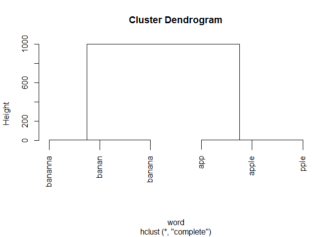
With this tree, it's now trivial to cut the tree and attribute the words to clusters.
clusters <- cutree(hc, h = 10) |>
  enframe(name = "word",
          value = "cluster")
clusters
#> # A tibble: 6 x 2
#>   word    cluster
#>   <chr>     <int>
#> 1 app           1
#> 2 apple         1
#> 3 banan         2
#> 4 banana        2
#> 5 bananna       2
#> 6 pple          1
Now we will want to use the counts per word. Let's prepare a new data frame for that. Again, since some words are only in col1, others only in col2, I'll duplicate df, extract col1 and col2, then bind them back into a single data frame.
counts_per_word <- df |>
  select(ends_with("2")) |>
  set_names(c("word", "count")) |>
  bind_rows(df |>
              select(ends_with("1")) |>
              set_names(c("word", "count"))) |>
  distinct()
counts_per_word
#> # A tibble: 6 x 2
#>   word    count
#>   <chr>   <dbl>
#> 1 pple        2
#> 2 app        50
#> 3 bananna     2
#> 4 banan      20
#> 5 apple     100
#> 6 banana    200
Finally, we have all our processed data in easy-to-use formats, we can simply combine it.
counts_per_word |>
  left_join(clusters,
            by = "word") |>
  group_by(cluster) |>
  summarize(main_word = word[which.max(count)],
            nb_words_in_cluster = n(),
            all_words = list(word),
            sum_counts = sum(count))
#> # A tibble: 2 x 5
#>   cluster main_word nb_words_in_cluster all_words sum_counts
#>     <int> <chr>                   <int> <list>         <dbl>
#> 1       1 apple                       3 <chr [3]>        152
#> 2       2 banana                      3 <chr [3]>        222
Created on 2022-03-18 by the reprex package (v2.0.1)
If you want exactly the format in your question, you can easily use unnest().
With a network approach
Since you already have a data frame that only contains distances for words from the same cluster, it may be simpler to use a network approach. For example:
library(tidyverse)
library(igraph)

df <- tibble(col1 = c("apple","apple","pple", "banana", "banana","bananna"),
             col2 = c("pple","app","app", "bananna", "banan", "banan"),
             distance = c(1,2,3,1,1,2),
             counts_col1 = c(100,100,2,200,200,2),
             counts_col2 = c(2,50,50,2,20,20))

gr <- df |>
  select(-starts_with("count")) |>
  rename(weight = distance) |>
  graph_from_data_frame()

plot(gr)
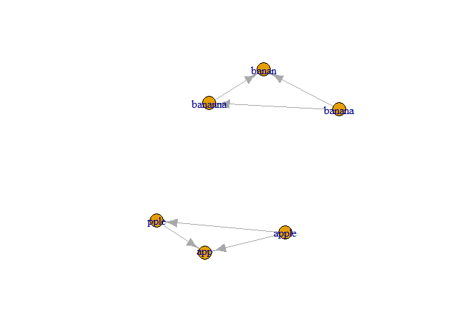
components(gr)$membership
#>   apple    pple  banana bananna     app   banan
#>       1       1       2       2       1       2
Created on 2022-03-18 by the reprex package (v2.0.1)
That replaces hclust() in a nice way, but you still have to find the highest count per cluster. You can use the code from above with counts_per_word.
However, I can't think of a way to easily use the count information as you provided it.