" Cannot convert object of class ggmapraster into a grob " Cartography with R

# # # - - CARTOGRAPHY | Representation of each genus on the map by a photo and its associated name 


# We will be satisfied with the Stammen format put under ggplot without more information on the relief otherwise it will be too heavy


# - - - - PACKAGES - - - -

library(ggplot2)
library(ggmap)
library(ggeasy)
library(mapdata)
library(maps)
library(marmap)
library(raster)
library(rasterVis)
library(cowplot)
library(prettymapr)
library(precrec)

- - - - - - - - - - - - - - - - - - - - - - - - - - - - - - - - - - - - - - - 
  
  
  # 1] Load the global map of Latin America 
  
  
  # We set the desired coordinates
  
  xlimsAmerica <- c(-100,-30)
  ylimsAmerica <- c(30,-56)
  
  # Retrieve the map in the desired mode 
  
  # -> (terrain-background i.e. nice google map without information)
  
  Amerique_Centrale <- get_stamenmap(bbox = c(left = min(xlimsAmérique),
                                              bottom = min(ylimsAmerica),
                                              right = max(xlimsAmerica),
                                              top = max(ylimsAmerica)),
                                     maptype = "terrain-background",
                                     zoom = 7) # important for detail (+ large number + detail)
  Amerique_Centrale<-ggmap(Amerique_Centrale)  
  
  ggmap(Amerique_Centrale)
  
  # save with save() in R.data format (will suffice to load() to get the file)
  
  save(Amerique_Centrale, file = "donnees_Amérique_Latine.RData") # save directly in the current directory
  
  # save with ggsave() 
  
  ggsave("Carte_Amerique_Latine.png", width = 12 , height = 20) # save by default the last plot made
  
  
  # - - - - - - - - - - - - - - - - - - - - - - - - - - - - - - - - - - - - - - - - - - - - - - - - 


  # 2] Load map of Guadeloupe 
  
  
  xlimsGuadeloupe <- c(-61.85,-61)
  ylimsGuadeloupe <- c(15.75,16.55)
  
  # we get the map according to the desired mode
  
  Guadeloupe <- get_stamenmap(bbox = c(left = min(xlimsGuadeloupe),
                                       bottom = min(ylimsGuadeloupe),
                                       right = max(xlimsGuadeloupe),
                                       top = max(ylimsGuadeloupe)),
                              maptype = "terrain-background", # type of map to represent
                              zoom = 11) # important for detail (+ large number + detail)
  Guadeloupe<-ggmap(Guadeloupe) 
  
  Guadeloupe


  # Save with save() in R.data format (load() will suffice to retrieve the file)
  
  save(Guadeloupe, file = "Guadeloupe.RData") # save directly in the current directory
  
  # save with ggsave() 
  
  ggsave("Guadeloupe.png", width = 15 , height = 12) # save by default the last plot made
  
  # - - - - - - - - - - - - - - - - - - - - - - - - - - - - - - - - - - - - - - - - - - - - - - - - 
  # 3] Load map of Madagascar  


  xlimsMadagascar <- c(40,55)
  ylimsMadagascar <- c(-10,-27)
  
  # get the map in the desired mode
  
  Madagascar <- get_stamenmap(bbox = c(left = min(xlimsMadagascar),
                                       bottom = min(ylimsMadagascar),
                                       right = max(xlimsMadagascar),
                                       top = max(ylimsMadagascar)),
                              maptype = "terrain-background", # type of map to represent
                              zoom = 8) # important for detail (+ large number + detail)
  Madagascar<-ggmap(Madagascar) 
  
  ggmap(Madagascar)


  save(Madagascar, file = "Madagascar.RData") # save directly to the current directory
  
  # save with ggsave() 
  
  ggsave("Madagascar.png", width = 15 , height = 12) # save by default the last plot made


  # - - - - - - - - - - - - - - - - - - - - - - - - - - - - - - - - - - - - - - - - - - - - - - - - 


  # 4] Plot everything in 1 (SOURCE: https://r-spatial.org/r/2018/10/25/ggplot2-sf-3.html ) 
  
  
  # The final map can be created using ggplot2 only, using 
  # cowplot and the draw_plot function, in which case it is easier to first define
  # the key figures for Guadeloupe and Madagascar:
  
  
  # We transform the maps into a ggplot object (Package ggplotify function as.ggplot) (? Useful?)
  
  library(ggplotify)
  
  Guadeloupe<-as.grob(Guadeloupe)
  Madagascar<-as.grob(Madagascar)


  (ratioGuadeloupe <- (2500000 - 200000) / (1600000 - (-2400000))
    
    ## [1] 0.575
    
    (ratioMadagascar <- (23 - 18) / (-154 - (-161))
      
      ## [1] 0.7142857
      
      ggdraw(Amerique_Centrale) +
        draw_plot(Guadeloupe, 
                  width = 0.26,
                  height = 0.26 * 10/6 * ratioGuadeloupe, 
                  x = 0.05,
                  y = 0.05)
      
      
      # ..... Ask the question so you don't have to do it on Guimp either


      # 
      

Hello !

This is my very first question on a forum dedicated to R and I hope it will go well, I am a biology student in Master and I don't practice R regularly

Here is the background:

I am trying to map on R and so far it works following a internet guide (Drawing beautiful maps programmatically with R, sf and ggplot2 — Part 3: Layouts), my goal is to make the kind of map visible on this link where several maps are combined (example of USA, Alaska & Hawaii in small).

So I loaded all the maps I wanted to show: Latin America, Madagascar and Guadeloupe where the last two maps would come in small.

I tried the two methods proposed on the website which are
(1) - function annotation_custom
(2) - using cowplot and the function draw_plot

My R code is attached,

Please be indulgent, my code is probably not up to the expectations of an official programmer as I am self-taught.

It would be a great help to me, thank you in advance, Thibaud
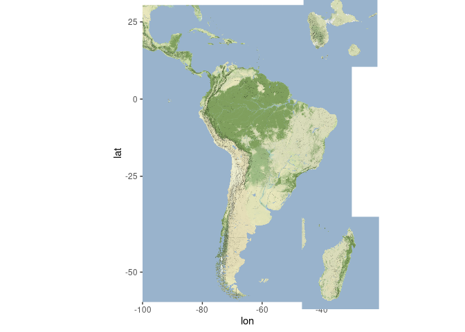
What's the question then? In current state the code (with small amendments) draws the South America and Guadeloupe together. Where is the issue?

BTW, please tidy your code, and use one naming convention: Amerique_Centrale != America_Central neither is Central_America called in ggdraw.

Regards,
Grzegorz

Thanks first of all,

I'm sorry because I don't code in English and I used a translator so there were some translation problems with Central-America , Amercia Centrale etc but it's ok here normally.

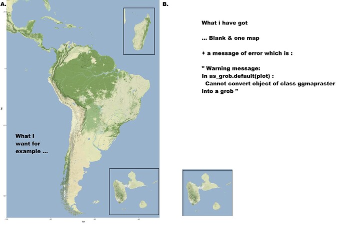
So I rewrote my question above to make sure it is understandable with a small image.... And it does not work as you can see so my question is

" I can I convert the ggmapraster format to grob or I dont' know to make it understandable for the fonction " draw_plot "

Is that clear ? I hope so

Thank you in advance,

It's working, I feel you are trying to do two things at a time. Let's try to get the data and visualize it.

library(ggplot2)
library(ggmap)
library(cowplot)

# 1] Load the global map of Latin America
xlimsAmerica <- c(-100, -30)
ylimsAmerica <- c(30, -56)

# Retrieve the map in the desired mode
# -> (terrain-background i.e. nice google map without information)

Amerique_Centrale <-
  get_stamenmap(
    bbox = c(
      left = min(xlimsAmerica),
      bottom = min(ylimsAmerica),
      right = max(xlimsAmerica),
      top = max(ylimsAmerica)
    ),
    maptype = "terrain-background",
    zoom = 6
  )
Amerique_Centrale <- ggmap(Amerique_Centrale)

If you wish to save the data for further use, then fine, however I would suggest to store the data before applying ggmap() to them.

# save with save() in R.data format (will suffice to load() to get the file)
save(Amerique_Centrale, file = "donnees_Amérique_Latine.RData")
# save with ggsave() 
# save by default the last plot made
ggsave("Carte_Amerique_Latine.png", width = 12 , height = 20)

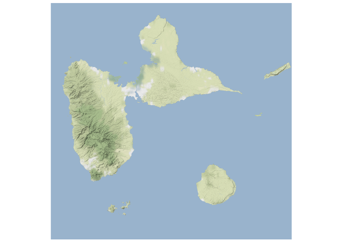
Let's load Guadeloupe:

# 2] Load map of Guadeloupe
xlimsGuadeloupe <- c(-61.85, -61)
ylimsGuadeloupe <- c(15.75, 16.55)

# we get the map according to the desired mode
Guadeloupe <- get_stamenmap(
  bbox = c(
    left = min(xlimsGuadeloupe),
    bottom = min(ylimsGuadeloupe),
    right = max(xlimsGuadeloupe),
    top = max(ylimsGuadeloupe)
  ),
  maptype = "terrain-background",
  # type of map to represent
  zoom = 11
)

Now a tricky part, we plot Guadeloupe with ggmap(), hovewer at the same time we remove the x and y axis labels and scales:

Guadeloupe <-  ggmap(Guadeloupe) +
  labs(x = "", y = "") +
  ggthemes::theme_map()
Guadeloupe

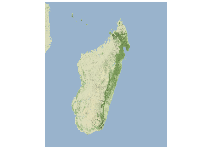
The same for Madagascar:

# 3] Load map of Madagascar
xlimsMadagascar <- c(40, 55)
ylimsMadagascar <- c(-10, -27)

# get the map in the desired mode
Madagascar <- get_stamenmap(
  bbox = c(
    left = min(xlimsMadagascar),
    bottom = min(ylimsMadagascar),
    right = max(xlimsMadagascar),
    top = max(ylimsMadagascar)
  ),
  maptype = "terrain-background",
  zoom = 8
)

Madagascar <- ggmap(Madagascar) +
  labs(x = "", y = "") +
  ggthemes::theme_map()

Madagascar

And let's plot everything as you tried, just using ggdraw() function:

# 4] Plot everything in 1 (SOURCE: https://r-spatial.org/r/2018/10/25/ggplot2-sf-3.html )

ratioGuadeloupe <- (2500000 - 200000) / (1600000 - (-2400000))
ratioMadagascar <- (23 - 18) / (-154 - (-161))

ggdraw(Amerique_Centrale) +
  draw_plot(
    Guadeloupe,
    width = 0.26,
    height = 0.26 * 10 / 6 * ratioGuadeloupe,
    x = 0.6,
    y = 0.78
  ) +
  draw_plot(
    Madagascar,
    width = 0.26,
    height = 0.26 * 10 / 6 * ratioMadagascar,
    x = 0.6,
    y = 0.05
  )

You can add borders to Madagascar and Guadeloupe like:

Guadeloupe <- ggmap(Guadeloupe) +
  labs(x = "", y = "") +
  ggthemes::theme_map() +
  theme(
    panel.border = element_rect(colour = "grey20", fill=NA, size=2)
  )

Back to your error with as.grob(). as.grob() function expects an object which is kind of ggplot. Therefore it shows an error, when trying to substitute map class data. Please have a look below:

We are importing tiles and create map

Guadeloupe <- get_stamenmap(
  bbox = c(
    left = min(xlimsGuadeloupe),
    bottom = min(ylimsGuadeloupe),
    right = max(xlimsGuadeloupe),
    top = max(ylimsGuadeloupe)
  ),
  maptype = "terrain-background",
  # type of map to represent
  zoom = 11
)

Running as.grob() now gives us an error:

as.grob(Guadeloupe)
#> Error in UseMethod("as.grob"): no applicable method for 'as.grob' applied to an object of class "c('ggmap', 'raster')"

However, plotting Guadeloupe with ggmap and reasigning it back to Guadeloupe makes things a bit different:

Guadeloupe <- ggmap(Guadeloupe) +
  labs(x = "", y = "") +
  ggthemes::theme_map() +
  theme(
    panel.border = element_rect(colour = "grey20", fill=NA, size=2)
  )
as.grob(Guadeloupe)
#> TableGrob (12 x 9) "layout": 18 grobs
#>     z         cells       name                                       grob
#> 1   0 ( 1-12, 1- 9) background     zeroGrob[plot.background..zeroGrob.36]
#> 2   5 ( 6- 6, 4- 4)     spacer                             zeroGrob[NULL]
#> 3   7 ( 7- 7, 4- 4)     axis-l         absoluteGrob[GRID.absoluteGrob.28]
[...]

Hope it makes sense,
Grzegorz
Created on 2022-02-04 by the reprex package (v2.0.1)

Unbelievable! Thank you, it works!

I have a last question concerning the code, do you understand this part concerning the dimensions of the Madagascar & Guadeloupe images for the Central American plot (code that I recovered on the Internet without having really understood it):

atioGuadeloupe <- (2500000 - 200000) / (1600000 - (-2400000))
ratioMadagascar <- (23 - 18) / (-154 - (-161))

Thanks again for the help! :slight_smile:

Generally speaking, it scales down the maps for both islands, but why in such mysterious way? I guess, someone used a different coordinate systems when calculated the ratioXXX -> that's the ratio between width and height of the island map, used later during final map composition.

Regards,
Grzegorz

OK then ! Thank you very much for your help !

This topic was automatically closed 7 days after the last reply. New replies are no longer allowed.

If you have a query related to it or one of the replies, start a new topic and refer back with a link.