Can I transform scales/axes from log to linear scale in ggplot2?

Hi everyone,

I am using log transformed data for my statistical analysis as it was not normally distributed and I wanted to run a few parametric tests. I have plotted the test results in various ways, mainly boxplots or barplots using ggplot2.
Obviously, the plot scales are also in log values in order to fit to the range of my results.
However, I would like to plot my results with a linear scale, because it would be easier to interpret the graphs.
So I wondered whether there is a way to just transform the log scale (and the plots) back into a linear scale in ggplot2? I know that it is possible to do it the other way round.
Or do I have to create all my plots just with my original non transformed data?

Very thankfull for any ideas or suggestions!

I'm not sure i understand the desired output ? like this ?

library(tidyverse)
library(scales)
mylogged_iris <- iris %>% select(Petal.Width,Sepal.Width) %>% mutate_all(log)

rexp2 <- function(x){round(exp(x),digits=2)}
g1<-ggplot(mylogged_iris,mapping=aes(Petal.Width,
                                 Sepal.Width)) + geom_point() 

  g1 + scale_y_continuous(trans = "exp",labels = rexp2)  + 
    scale_x_continuous(trans="exp",limits = c(.01,1.1),labels = rexp2)
1 Like

Thanks for your quick reply! Great, that was basically what I was looking for, though I thought there would be an easier way of doing it (well, it is actually easy when you know what you do).

Your code works well with a small dummy data set, but it doesnt work with my original data.

I have also tried a small subset of my data, which I will include here, but I always get the error message

Error in if (zero_range(as.numeric(limits))) { :
missing value where TRUE/FALSE needed
In addition: Warning messages:
1: Continuous x aesthetic -- did you forget aes(group=...)?
2: In self$trans$inverse(limits) : NaNs produced

Any suggestions what could cause this?

I use the following code, but have removed the coding for the x axis, because I would like to keep it as it is.

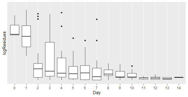
data$logResidues=log(data$Residues)
attach (data)
data$Day<-as.factor(data$Day)
data$Matrix<-as.factor(data$Matrix)

library(ggplot2)
library(scales)

rexp2 <- function(x){round(exp(x),digits=2)}
ggplot(data, aes(x=Day, y=logResidues)) + 
  geom_boxplot()
 scale_y_continuous(trans = "exp",labels = rexp2)

My dataset:

data <- wrapr::build_frame( "Day" , "Residues" | 0 , 1421 | 0 , 858.1 | 0 , 1582 | 0 , 1332 | 0 , 1653 | 0 , 754.9 | 1 , 452.9 | 1 , 379.8 | 1 , 230.4 | 1 , 333 | 1 , 292.6 | 1 , 322.6 | 2 , 163.4 | 2 , 154.9 | 2 , 179.1 | 2 , 127.6 | 2 , 156.2 | 2 , 122.3 | 3 , 87.14 | 3 , 82.05 | 3 , 84.39 | 3 , 74.28 | 3 , 101.5 | 3 , 85.38 | 4 , 48.99 | 4 , 50.71 | 4 , 41.3 | 4 , 53.23 | 4 , 107.8 | 4 , 50.63 | 5 , 59.26 | 5 , 58.54 | 5 , 56.2 | 5 , 58.49 | 6 , 66.49 | 6 , 52.75 | 6 , 79.95 | 1 , 492.2 | 1 , 437.9 | 1 , 573.4 | 2 , 190.9 | 2 , 155.1 | 2 , 315.3 | 2 , 132.9 | 3 , 78.97 | 3 , 132 | 3 , 177.8 | 3 , 60.87 | 4 , 59.07 | 4 , 45.94 | 4 , 44.37 | 4 , 135.1 | 4 , 152.4 | 5 , 43.72 | 5 , 34.05 | 5 , 84.22 | 5 , 28.46 | 6 , 30.6 | 6 , 56.88 | 6 , 51.16 | 6 , 30.71 | 7 , 26.66 | 7 , 79.67 | 7 , 122 | 8 , 34.42 | 8 , 23.23 | 2 , 49.25 | 2 , 32.27 | 2 , 22.96 | 3 , 18.8 | 3 , 16.99 | 3 , 28.35 | 4 , 10.81 | 4 , 42.52 | 4 , 11.95 | 4 , 31.42 | 4 , 16.47 | 5 , 12.46 | 5 , 15.86 | 5 , 13.45 | 5 , 14.81 | 5 , 13.98 | 6 , 20.04 | 6 , 19.78 | 6 , 16.42 | 6 , 19.67 | 6 , 13.3 | 7 , 7.042 | 7 , 8.863 | 7 , 10.23 | 7 , 15.87 | 7 , 8.164 | 8 , 7.051 | 8 , 9.886 | 8 , 13.54 | 8 , 10.36 | 8 , 10.72 | 9 , 7.033 | 9 , 7.459 | 9 , 7.374 | 9 , 10.78 | 9 , 7.259 | 10 , 6.453 | 10 , 7.418 | 10 , 9.636 | 5 , 28.36 | 5 , 11.63 | 6 , 13.13 | 6 , 16.65 | 6 , 15.58 | 7 , 25.49 | 7 , 39.92 | 8 , 14.52 | 8 , 22.11 | 8 , 22.26 | 8 , 20.3 | 8 , 12.99 | 9 , 6.846 | 9 , 10.38 | 9 , 21.94 | 9 , 32.48 | 9 , 30.77 | 9 , 24.83 | 10 , 22.93 | 10 , 29.44 | 10 , 20.31 | 10 , 6.09 | 10 , 6.506 | 10 , 7.211 | 11 , 6.324 | 11 , 6.366 | 11 , 4.742 | 11 , 6.687 | 11 , 3.891 | 11 , 9.163 | 12 , 12.84 | 12 , 7.168 | 12 , 5.39 | 12 , 2.624 | 12 , 2.853 | 13 , 6.973 | 13 , 6.773 | 13 , 3.683 | 13 , 2.647 | 14 , 8.173 | 14 , 0.2251 | 14 , 5.83 | 0 , 204.5 | 0 , 220.6 | 0 , 250.9 | 1 , 140.8 | 1 , 306 | 1 , 377.5 | 1 , 277.7 | 1 , 271.5 | 2 , 33.07 | 2 , 33.7 | 2 , 54.25 | 2 , 34.94 | 2 , 21.72 | 3 , 8.549 | 3 , 9.943 | 3 , 12.1 | 3 , 16.22 | 4 , 10.65 | 4 , 10.46 | 4 , 12.72 | 4 , 10.1 | 5 , 4.369 | 5 , 18.32 | 5 , 18.16 | 5 , 7.83 | 2 , 2.627 | 2 , 2.111 | 2 , 1.621 | 3 , 3.372 | 3 , 9.415 | 3 , 1.58 | 3 , 1.735 | 4 , 2.491 | 4 , 1.333 | 4 , 4.534 | 4 , 1.643 | 5 , 3.102 | 5 , 1.286 | 5 , 0.5211 | 5 , 3.277 | 5 , 2.605 | 6 , 2.754 | 6 , 1.806 | 6 , 4.556 | 6 , 2.336 | 6 , 0.9231 | 7 , 0.9389 | 7 , 0.2155 | 7 , 0.4852 | 7 , 2.321 | 7 , 0.4026 | 8 , 0.3178 | 8 , 0.01145 | 8 , 0.4557 | 8 , 1.533 | 8 , 0.4227 | 5 , 0.3688 | 5 , 0.4078 | 6 , 0.5388 | 6 , 0.9522 | 6 , 1.756 | 7 , 0.5251 | 7 , 0.1848 | 7 , 1.12 | 7 , 2.056 | 8 , 0.3929 | 8 , 0.2678 | 8 , 1.599 | 8 , 0.8073 | 8 , 0.6894 | 9 , 2.482 | 9 , 0.9661 | 9 , 0.2109 | 9 , 0.6317 | 9 , 2.527 | 10 , 0.619 | 10 , 1.802 | 10 , 2.792 | 10 , 0.9921 | 10 , 0.4267 | 11 , 0.1299 | 11 , 2.834 | 11 , 1.986 | 11 , 0.7228 | 11 , 0.7338 | 12 , 0.3672 | 12 , 0.687 | 12 , 0.3285 | 13 , 2.387 | 13 , 0.2714 | 13 , 0.1297 | 14 , 0.3096 | 14 , 0.3483 | 14 , 0.2438 | 0 , 92 | 0 , 89.9 | 0 , 184.2 | 0 , 129 | 1 , 62.15 | 1 , 114.1 | 1 , 82.58 | 1 , 93.36 | 1 , 49.24 | 2 , 31.79 | 2 , 22.33 | 2 , 21.24 | 2 , 19.59 | 2 , 24.07 | 3 , 25.98 | 3 , 16.64 | 3 , 22.93 | 3 , 23.51 | 4 , 19.61 | 4 , 14.63 | 4 , 11.59 | 4 , 21.88 | 5 , 14.88 | 5 , 5.833 | 5 , 11.13 | 5 , 15.03 | 2 , 1.885 | 2 , 1.5 | 2 , 1.68 | 3 , 1.664 | 3 , 1.866 | 3 , 1.485 | 4 , 1.617 | 4 , 1.605 | 4 , 2.492 | 4 , 1.987 | 5 , 1.729 | 5 , 1.992 | 5 , 1.858 | 5 , 2.211 | 6 , 1.996 | 6 , 1.949 | 6 , 1.841 | 6 , 1.67 | 7 , 1.238 | 7 , 1.441 | 7 , 1.724 | 7 , 1.355 | 8 , 0.1542 | 8 , 0.5447 | 8 , 0.2885 | 8 , 0.8485 | 5 , 0.498 | 5 , 0.1773 | 6 , 0.3504 | 6 , 1.186 | 6 , 0.376 | 7 , 0.5741 | 7 , 0.7487 | 8 , 0.3315 | 8 , 0.3668 | 8 , 0.3816 | 8 , 0.7679 | 9 , 0.4884 | 9 , 0.3739 | 9 , 1.265 | 9 , 0.4569 | 10 , 0.4275 | 10 , 0.3761 | 10 , 0.4069 | 10 , 0.3294 | 13 , 0.2735 | 13 , 0.1601 | 13 , 0.6603 | 14 , 0.3572 | 14 , 0.3146 | 14 , 0.4143 | 0 , 651.9 | 0 , 936.9 | 0 , 759.1 | 0 , 763.6 | 1 , 693.1 | 1 , 1181 | 1 , 551.5 | 1 , 638.3 | 2 , 465.8 | 2 , 1409 | 2 , 608.6 | 2 , 692.1 | 2 , 968.8 | 3 , 713 | 3 , 963.7 | 3 , 656.5 | 3 , 865.4 | 3 , 1052 | 4 , 1212 | 4 , 1186 | 4 , 1222 | 4 , 715.9 | 4 , 735.6 | 5 , 769.2 | 5 , 1339 | 5 , 653.7 | 5 , 665 | 2 , 442.4 | 2 , 618 | 2 , 728.4 | 3 , 618.9 | 3 , 800.1 | 3 , 526.1 | 4 , 1118 | 4 , 830.8 | 4 , 797.2 | 4 , 994.2 | 4 , 926 | 5 , 896.6 | 5 , 902.3 | 5 , 1118 | 5 , 815.6 | 5 , 1063 | 6 , 435.4 | 6 , 472.6 | 6 , 971.5 | 6 , 775.3 | 6 , 1093 | 7 , 355.6 | 7 , 967.8 | 7 , 698.7 | 7 , 978.1 | 7 , 1058 | 8 , 622 | 8 , 1327 | 8 , 1318 | 8 , 1009 | 8 , 604.6 | 5 , 648.5 | 6 , 1110 | 6 , 1458 | 6 , 778.9 | 7 , 764.1 | 7 , 1184 | 7 , 962.7 | 7 , 581.1 | 7 , 888.1 | 8 , 687.4 | 8 , 913.1 | 8 , 513 | 8 , 618.2 | 8 , 497.4 | 9 , 959.7 | 9 , 730.6 | 9 , 733 | 9 , 886.3 | 9 , 894.7 | 9 , 906.3 | 10 , 520.5 | 10 , 1037 | 10 , 568.1 | 10 , 671.7 | 10 , 388.8 | 10 , 534.3 | 11 , 717.4 | 11 , 896.1 | 11 , 917.2 | 11 , 774 | 11 , 1208 | 11 , 529.9 | 12 , 850.8 | 12 , 803.7 | 12 , 1141 | 13 , 1383 | 13 , 861.1 | 13 , 739 )

data

structure(list(Day = c(0, 0, 0, 0, 0, 0, 1, 1, 1, 1, 1, 1, 2, 
2, 2, 2, 2, 2, 3, 3, 3, 3, 3, 3, 4, 4, 4, 4, 4, 4, 5, 5, 5, 5, 
6, 6, 6, 1, 1, 1, 2, 2, 2, 2, 3, 3, 3, 3, 4, 4, 4, 4, 4, 5, 5, 
5, 5, 6, 6, 6, 6, 7, 7, 7, 8, 8, 2, 2, 2, 3, 3, 3, 4, 4, 4, 4, 
4, 5, 5, 5, 5, 5, 6, 6, 6, 6, 6, 7, 7, 7, 7, 7, 8, 8, 8, 8, 8, 
9, 9, 9, 9, 9, 10, 10, 10, 5, 5, 6, 6, 6, 7, 7, 8, 8, 8, 8, 8, 
9, 9, 9, 9, 9, 9, 10, 10, 10, 10, 10, 10, 11, 11, 11, 11, 11, 
11, 12, 12, 12, 12, 12, 13, 13, 13, 13, 14, 14, 14, 0, 0, 0, 
1, 1, 1, 1, 1, 2, 2, 2, 2, 2, 3, 3, 3, 3, 4, 4, 4, 4, 5, 5, 5, 
5, 2, 2, 2, 3, 3, 3, 3, 4, 4, 4, 4, 5, 5, 5, 5, 5, 6, 6, 6, 6, 
6, 7, 7, 7, 7, 7, 8, 8, 8, 8, 8, 5, 5, 6, 6, 6, 7, 7, 7, 7, 8, 
8, 8, 8, 8, 9, 9, 9, 9, 9, 10, 10, 10, 10, 10, 11, 11, 11, 11, 
11, 12, 12, 12, 13, 13, 13, 14, 14, 14, 0, 0, 0, 0, 1, 1, 1, 
1, 1, 2, 2, 2, 2, 2, 3, 3, 3, 3, 4, 4, 4, 4, 5, 5, 5, 5, 2, 2, 
2, 3, 3, 3, 4, 4, 4, 4, 5, 5, 5, 5, 6, 6, 6, 6, 7, 7, 7, 7, 8, 
8, 8, 8, 5, 5, 6, 6, 6, 7, 7, 8, 8, 8, 8, 9, 9, 9, 9, 10, 10, 
10, 10, 13, 13, 13, 14, 14, 14, 0, 0, 0, 0, 1, 1, 1, 1, 2, 2, 
2, 2, 2, 3, 3, 3, 3, 3, 4, 4, 4, 4, 4, 5, 5, 5, 5, 2, 2, 2, 3, 
3, 3, 4, 4, 4, 4, 4, 5, 5, 5, 5, 5, 6, 6, 6, 6, 6, 7, 7, 7, 7, 
7, 8, 8, 8, 8, 8, 5, 6, 6, 6, 7, 7, 7, 7, 7, 8, 8, 8, 8, 8, 9, 
9, 9, 9, 9, 9, 10, 10, 10, 10, 10, 10, 11, 11, 11, 11, 11, 11, 
12, 12, 12, 13, 13, 13), Residues = c(1421, 858.1, 1582, 1332, 
1653, 754.9, 452.9, 379.8, 230.4, 333, 292.6, 322.6, 163.4, 154.9, 
179.1, 127.6, 156.2, 122.3, 87.14, 82.05, 84.39, 74.28, 101.5, 
85.38, 48.99, 50.71, 41.3, 53.23, 107.8, 50.63, 59.26, 58.54, 
56.2, 58.49, 66.49, 52.75, 79.95, 492.2, 437.9, 573.4, 190.9, 
155.1, 315.3, 132.9, 78.97, 132, 177.8, 60.87, 59.07, 45.94, 
44.37, 135.1, 152.4, 43.72, 34.05, 84.22, 28.46, 30.6, 56.88, 
51.16, 30.71, 26.66, 79.67, 122, 34.42, 23.23, 49.25, 32.27, 
22.96, 18.8, 16.99, 28.35, 10.81, 42.52, 11.95, 31.42, 16.47, 
12.46, 15.86, 13.45, 14.81, 13.98, 20.04, 19.78, 16.42, 19.67, 
13.3, 7.042, 8.863, 10.23, 15.87, 8.164, 7.051, 9.886, 13.54, 
10.36, 10.72, 7.033, 7.459, 7.374, 10.78, 7.259, 6.453, 7.418, 
9.636, 28.36, 11.63, 13.13, 16.65, 15.58, 25.49, 39.92, 14.52, 
22.11, 22.26, 20.3, 12.99, 6.846, 10.38, 21.94, 32.48, 30.77, 
24.83, 22.93, 29.44, 20.31, 6.09, 6.506, 7.211, 6.324, 6.366, 
4.742, 6.687, 3.891, 9.163, 12.84, 7.168, 5.39, 2.624, 2.853, 
6.973, 6.773, 3.683, 2.647, 8.173, 0.2251, 5.83, 204.5, 220.6, 
250.9, 140.8, 306, 377.5, 277.7, 271.5, 33.07, 33.7, 54.25, 34.94, 
21.72, 8.549, 9.943, 12.1, 16.22, 10.65, 10.46, 12.72, 10.1, 
4.369, 18.32, 18.16, 7.83, 2.627, 2.111, 1.621, 3.372, 9.415, 
1.58, 1.735, 2.491, 1.333, 4.534, 1.643, 3.102, 1.286, 0.5211, 
3.277, 2.605, 2.754, 1.806, 4.556, 2.336, 0.9231, 0.9389, 0.2155, 
0.4852, 2.321, 0.4026, 0.3178, 0.01145, 0.4557, 1.533, 0.4227, 
0.3688, 0.4078, 0.5388, 0.9522, 1.756, 0.5251, 0.1848, 1.12, 
2.056, 0.3929, 0.2678, 1.599, 0.8073, 0.6894, 2.482, 0.9661, 
0.2109, 0.6317, 2.527, 0.619, 1.802, 2.792, 0.9921, 0.4267, 0.1299, 
2.834, 1.986, 0.7228, 0.7338, 0.3672, 0.687, 0.3285, 2.387, 0.2714, 
0.1297, 0.3096, 0.3483, 0.2438, 92, 89.9, 184.2, 129, 62.15, 
114.1, 82.58, 93.36, 49.24, 31.79, 22.33, 21.24, 19.59, 24.07, 
25.98, 16.64, 22.93, 23.51, 19.61, 14.63, 11.59, 21.88, 14.88, 
5.833, 11.13, 15.03, 1.885, 1.5, 1.68, 1.664, 1.866, 1.485, 1.617, 
1.605, 2.492, 1.987, 1.729, 1.992, 1.858, 2.211, 1.996, 1.949, 
1.841, 1.67, 1.238, 1.441, 1.724, 1.355, 0.1542, 0.5447, 0.2885, 
0.8485, 0.498, 0.1773, 0.3504, 1.186, 0.376, 0.5741, 0.7487, 
0.3315, 0.3668, 0.3816, 0.7679, 0.4884, 0.3739, 1.265, 0.4569, 
0.4275, 0.3761, 0.4069, 0.3294, 0.2735, 0.1601, 0.6603, 0.3572, 
0.3146, 0.4143, 651.9, 936.9, 759.1, 763.6, 693.1, 1181, 551.5, 
638.3, 465.8, 1409, 608.6, 692.1, 968.8, 713, 963.7, 656.5, 865.4, 
1052, 1212, 1186, 1222, 715.9, 735.6, 769.2, 1339, 653.7, 665, 
442.4, 618, 728.4, 618.9, 800.1, 526.1, 1118, 830.8, 797.2, 994.2, 
926, 896.6, 902.3, 1118, 815.6, 1063, 435.4, 472.6, 971.5, 775.3, 
1093, 355.6, 967.8, 698.7, 978.1, 1058, 622, 1327, 1318, 1009, 
604.6, 648.5, 1110, 1458, 778.9, 764.1, 1184, 962.7, 581.1, 888.1, 
687.4, 913.1, 513, 618.2, 497.4, 959.7, 730.6, 733, 886.3, 894.7, 
906.3, 520.5, 1037, 568.1, 671.7, 388.8, 534.3, 717.4, 896.1, 
917.2, 774, 1208, 529.9, 850.8, 803.7, 1141, 1383, 861.1, 739
)), row.names = c(NA, -414L), class = c("tbl_df", "tbl", "data.frame"
))

code


data$logResidues=log(data$Residues)
data$Day<-as.factor(data$Day)
 
library(ggplot2)
library(scales)

rexp2 <- function(x){round(exp(x),digits=2)}
ggplot(data, aes(x=Day, y=logResidues)) + 
  geom_boxplot() +
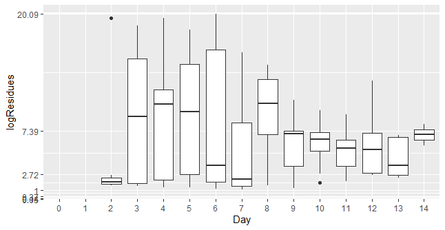
  scale_y_continuous(trans = "exp",limits = c(.001,2),labels = rexp2)

ggplot(data, aes(x=Day, y=logResidues)) + 
  geom_boxplot() +
  scale_y_continuous(trans = "exp",limits = c(.001,3),labels = rexp2)
Thanks for the reply!
Could you explain what limits= c(0.001, 3) stands for?

When using your code the boxplots on Day 0 and 1 are not visible.

grafik

They do appear when I change the max limit to 5 , however I have to remove the breaks in order to make the code work, which means my y axis disappears.

ggplot(data, aes(x=Day, y=logResidues)) + 
  geom_boxplot()+
  scale_y_continuous(trans = "exp",limits = c(0,5), labels= rexp2, breaks=NULL)

grafik

Do you know how I could get the breaks and y axis labels back?

Many thanks for your help!

I'm pretty sure ggplot2 boplots just werent designed to work with log scales, so will give odd behaviour.
I think there is some in-depth discussion of what you can try here.

This topic was automatically closed 21 days after the last reply. New replies are no longer allowed.