The way you posted your data makes to hard to use. I put it in a csv file and after a little editing ended up with this:
      ra    dark   col.0    MUT3    MUT7    MUT8   MUT11    MUTB
1   0.29 1.14270 1.07935 0.92150 0.95455 1.00930      NA      NA
2     NA 1.03948 0.97160 1.05136 0.72216 0.64828 0.89825 1.11400
3     NA 1.10108 1.14012 1.17932 0.97376 1.08220 1.18640 1.12828
4   0.80      NA      NA      NA      NA      NA      NA      NA
5     NA      NA      NA      NA      NA      NA      NA      NA
6     NA      NA      NA      NA      NA      NA      NA      NA
7     NA      NA      NA      NA      NA      NA      NA      NA
8   2.00 1.39315 1.07410      NA 1.23505      NA 1.00275 1.29445
9     NA 1.05380 0.65850 0.95685 0.88160 0.75710 0.77700 1.08480
10    NA 1.07144 0.74720 0.86424 0.92396 0.94128 0.75144 1.04908
11  3.80 0.86764 0.58508      NA 0.69488 0.74408 0.72272 1.16696
12    NA 1.28232 0.93884 0.98236 0.86272 1.02316 0.85916 1.13588
13    NA 0.88712 0.56972      NA 0.99988 0.77440 0.72200 1.17872
14 10.00 0.78900 0.49488 0.65032 0.65148 0.78180 0.53324 0.87880
15    NA 1.19616 0.80104 1.11956 0.83084 1.05012 0.80300 1.18224
16    NA 1.03348 0.64452 0.73748 0.90344 0.96140 0.60148 1.11060
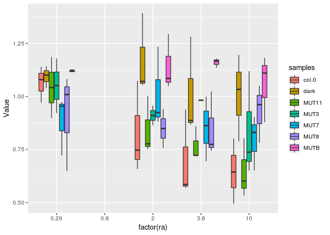
It seems that your repeated measurements are designated by having NA in the first column. I used the fill() function to put the actual values in the first column then pivoted the data to a long format and made a box plot. I think a box plot is not a good choice for this plot. With only three values per condition, the box plot gives the impression of having more data than are actually available. The first and third quartiles are not very well determined from such a small sample. Also, the x axis is categorical in a box plot but your x values are continuous values.
DF <- read.csv("~/R/Play/Dummy.csv", sep = " ")
library(tidyr)
DF <- fill(DF, ra, .direction = "down")
DFlong <- DF %>% pivot_longer(cols = -"ra", names_to = "samples", values_to = "Value")
DFlong
#> # A tibble: 112 × 3
#>       ra samples  Value
#>    <dbl> <chr>    <dbl>
#>  1  0.29 dark     1.14
#>  2  0.29 col.0    1.08
#>  3  0.29 MUT3     0.921
#>  4  0.29 MUT7     0.955
#>  5  0.29 MUT8     1.01
#>  6  0.29 MUT11   NA
#>  7  0.29 MUTB    NA
#>  8  0.29 dark     1.04
#>  9  0.29 col.0    0.972
#> 10  0.29 MUT3     1.05
#> # … with 102 more rows
library(ggplot2)
ggplot(DFlong, aes(x = factor(ra), y = Value, fill = samples)) + geom_boxplot()
#> Warning: Removed 34 rows containing non-finite values (stat_boxplot).

Created on 2022-04-19 by the reprex package (v0.2.1)
A better way to post data is with the dput() function The output of dput(DF) is
structure(list(ra = c(0.29, NA, NA, 0.8, NA, NA, NA, 2, NA, NA,
3.8, NA, NA, 10, NA, NA), dark = c(1.1427, 1.03948, 1.10108,
NA, NA, NA, NA, 1.393149999999, 1.0538, 1.071439999999, 0.867639999999,
1.282319999999, 0.887119999999, 0.788999999999, 1.19616, 1.03348
), col.0 = c(1.07935, 0.9716, 1.1401199999999, NA, NA, NA, NA,
1.0741, 0.6585, 0.7472, 0.58508, 0.9388399999999, 0.56972, 0.4948799999999,
0.8010399999999, 0.64452), MUT3 = c(0.921499999999, 1.051359999999,
1.179319999999, NA, NA, NA, NA, NA, 0.956849999999, 0.864239999999,
NA, 0.98236, NA, 0.65032, 1.119559999999, 0.737479999999), MUT7 = c(0.95455,
0.722159999999, 0.97376, NA, NA, NA, NA, 1.235049999999, 0.8816,
0.923959999999, 0.694879999999, 0.86272, 0.999879999999, 0.651479999999,
0.830839999999, 0.903439999999), MUT8 = c(1.0093, 0.64827999999,
1.0822, NA, NA, NA, NA, NA, 0.7571, 0.94127999999, 0.74407999999,
1.02315999999, 0.77439999999, 0.7818, 1.05012, 0.96139999999),
    MUT11 = c(NA, 0.89825, 1.18639999999, NA, NA, NA, NA, 1.00275,
    0.777, 0.75144, 0.72272, 0.85915999999, 0.72199999999, 0.53323999999,
    0.80299999999, 0.60148), MUTB = c(NA, 1.114, 1.12827999999,
    NA, NA, NA, NA, 1.29444999999, 1.0848, 1.04908, 1.16696,
    1.13587999999, 1.17872, 0.8788, 1.18224, 1.11059999999)), class = "data.frame", row.names = c(NA, -16L))
That can be easily used to recreate the data in my csv file by just copying the structure() call and assigning its value to DF.

