bar plot according to given data

Hi everybody, I need help with my bar plot (for my thesis). I wanted to make it a plot according to the sequence of the data, but instead, it was arranged from lowest to highest. Thank you so much.

library(readr)
library(ggplot2)
library(tidyverse)
library(dplyr)
library(reshape2)
library(wesanderson)

library(rstatix)
library(ggpubr)
library(plyr)
library(datarium)
library(summariser)
library(ggrepel)
library(ggprism)
library(patchwork)
library(magrittr)

AptaC10<-data.frame(Purification=c("HPLC","HPLC","HPLC","HPLC","HPLC","HPLC","HPLC","HPLC","HPLC","HPLC","HPLC","HPLC","HPLC","HPLC","HPLC","HPLC","HPLC","HPLC",
"Original","Original","Original","Original","Original","Original","Original","Original","Original","Original","Original","Original","Original","Original","Original","Original","Original","Original"),
time=c("48","48","48","48","48","48","48","48","48","96","96","96","96","96","96","96","96","96","48","48","48","48","48","48","48","48","48","96","96","96","96","96","96","96","96","96"),
con=c("0","5","10","25","50","100","250","500","750","0","5","10","25","50","100","250","500","750","0","5","10","25","50","100","250","500","750","0","5","10","25","50","100","250","500","750"),
bgrowth=c("0.6571630","0.6735407","0.6633407","0.6759000","0.7049111","0.7174444","0.6808407","0.6397963","0.6485444","0.6509333","0.6478444","0.6346000","0.6307741","0.6254704","0.5887815",
"0.5769222","0.5469444","0.5809481","0.6571630","0.6887704","0.6746222","0.6781222","0.7078963","0.7092037","0.6641481","0.6258000","0.6446926","0.6509333", "0.6690037","0.6414148","0.6352926","0.6206370",
"0.5787037","0.5591593","0.5363593","0.5673148"))

ggplot(data = AptaC10, mapping = aes(x=time, y=bgrowth, fill=con)) +
geom_bar(stat="identity", position = "dodge") +
facet_grid(~Purification)+
theme_bw()+
scale_fill_manual(name = "Concentration\n(ppm)",
values = c("0" = "black", "5" = "red", "10"= "purple",
"25"="blue", "50"= "darkgreen", "100"= "orange",
"250"= "skyblue", "500"="maroon", "750"="violet"))
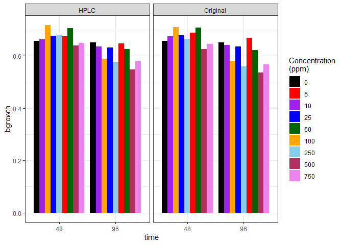
Is this what you are looking for? All I did is change the bgrowth column from being characters to numbers.

library(ggplot2)
library(dplyr)
AptaC10<-data.frame(Purification=c("HPLC","HPLC","HPLC","HPLC","HPLC","HPLC","HPLC","HPLC","HPLC","HPLC","HPLC","HPLC","HPLC","HPLC","HPLC","HPLC","HPLC","HPLC",
                                   "Original","Original","Original","Original","Original","Original","Original","Original","Original","Original","Original","Original","Original","Original","Original","Original","Original","Original"),
                    time=c("48","48","48","48","48","48","48","48","48","96","96","96","96","96","96","96","96","96","48","48","48","48","48","48","48","48","48","96","96","96","96","96","96","96","96","96"),
                    con=c("0","5","10","25","50","100","250","500","750","0","5","10","25","50","100","250","500","750","0","5","10","25","50","100","250","500","750","0","5","10","25","50","100","250","500","750"),
                    bgrowth=c("0.6571630","0.6735407","0.6633407","0.6759000","0.7049111","0.7174444","0.6808407","0.6397963","0.6485444","0.6509333","0.6478444","0.6346000","0.6307741","0.6254704","0.5887815",
                              "0.5769222","0.5469444","0.5809481","0.6571630","0.6887704","0.6746222","0.6781222","0.7078963","0.7092037","0.6641481","0.6258000","0.6446926","0.6509333", "0.6690037","0.6414148","0.6352926","0.6206370",
                              "0.5787037","0.5591593","0.5363593","0.5673148"))


AptaC10 <- AptaC10 |> mutate(bgrowth=as.numeric(bgrowth))
ggplot(data = AptaC10, mapping = aes(x=time, y=bgrowth, fill=con)) +
  geom_bar(stat="identity", position = "dodge") +
  facet_grid(~Purification)+
  theme_bw()+
  scale_fill_manual(name = "Concentration\n(ppm)",
                    values = c("0" = "black", "5" = "red", "10"= "purple",
                               "25"="blue", "50"= "darkgreen", "100"= "orange",
                               "250"= "skyblue", "500"="maroon", "750"="violet"))
Created on 2022-07-02 by the reprex package (v2.0.1)

1 Like

Changing the format of the con column gives better ordering of the colors in the plot.

AptaC10 <- AptaC10 |> mutate(bgrowth=as.numeric(bgrowth),
                             con=formatC(as.numeric(con),width=3,flag = "0"))
ggplot(data = AptaC10, mapping = aes(x=time, y=bgrowth, fill=con)) +
  geom_bar(stat="identity", position = "dodge") +
  facet_grid(~Purification)+
  theme_bw()+
  scale_fill_manual(name = "Concentration\n(ppm)",
                    values = c("000" = "black", "005" = "red", "010"= "purple",
                               "025"="blue", "050"= "darkgreen", "100"= "orange",
                               "250"= "skyblue", "500"="maroon", "750"="violet"))
1 Like

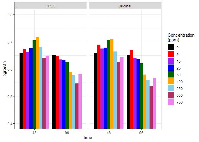
Hi @FJCC, thank you for your input on a solution to my problem, however, I have observed that the legends got changed from "0" to "000" and so on. Also, the values of the bgrowth start from the minimum of 0.4038 and maximum of 0.850556, how will I make it appear in the graph? Thanks.

Rex

I modified the code to change the labels in the legend and to show a set range of the y axis.

library(ggplot2)
library(dplyr)

AptaC10<-data.frame(Purification=c("HPLC","HPLC","HPLC","HPLC","HPLC","HPLC","HPLC","HPLC","HPLC","HPLC","HPLC","HPLC","HPLC","HPLC","HPLC","HPLC","HPLC","HPLC",
                                   "Original","Original","Original","Original","Original","Original","Original","Original","Original","Original","Original","Original","Original","Original","Original","Original","Original","Original"),
                    time=c("48","48","48","48","48","48","48","48","48","96","96","96","96","96","96","96","96","96","48","48","48","48","48","48","48","48","48","96","96","96","96","96","96","96","96","96"),
                    con=c("0","5","10","25","50","100","250","500","750","0","5","10","25","50","100","250","500","750","0","5","10","25","50","100","250","500","750","0","5","10","25","50","100","250","500","750"),
                    bgrowth=c("0.6571630","0.6735407","0.6633407","0.6759000","0.7049111","0.7174444","0.6808407","0.6397963","0.6485444","0.6509333","0.6478444","0.6346000","0.6307741","0.6254704","0.5887815",
                              "0.5769222","0.5469444","0.5809481","0.6571630","0.6887704","0.6746222","0.6781222","0.7078963","0.7092037","0.6641481","0.6258000","0.6446926","0.6509333", "0.6690037","0.6414148","0.6352926","0.6206370",
                              "0.5787037","0.5591593","0.5363593","0.5673148"))


AptaC10 <- AptaC10 |> mutate(bgrowth=as.numeric(bgrowth),
                             con=formatC(as.numeric(con),width=3,flag = "0"))
ggplot(data = AptaC10, mapping = aes(x=time, y=bgrowth, fill=con)) +
  geom_bar(stat="identity", position = "dodge") +
  facet_grid(~Purification)+
  theme_bw()+
  scale_fill_manual(name = "Concentration\n(ppm)",
                    values = c("000" = "black", "005" = "red", "010"= "purple",
                               "025"="blue", "050"= "darkgreen", "100"= "orange",
                               "250"= "skyblue", "500"="maroon", "750"="violet"),
                    labels=c("0","5","10","25","50","100","250","500","750"))+
  coord_cartesian(ylim=c(0.4,0.8))

Created on 2022-07-03 by the reprex package (v2.0.1)

1 Like

The values of bgrowth are already the means, my next worry is how to show the standard deviation out of it?

Thanks again,

Rex

The ggplot2 package includes a geom_errorbar. Take a look at that. If you get stuck, please post the data containing the standard deviations and the code you have tried.

1 Like

Dear @FJCC , here is my data, as explained previously the values are not showing the standard deviation, because when I run the code,
AptaC10run123<-(read.csv("~/R/Data Analysis/MSc ARTs/Summary/June 2022/AptataC10RawPur.4896H.csv", stringsAsFactors=TRUE))
AptaC10 <- aggregate(bgrowth ~ con + time + Purification, AptaC10run123,mean)

summary<-AptaC10run123 %>%
group_by(time) %>%
get_summary_stats(bgrowth, type = "mean_sd")
data.frame(summary)

It only gives me the following results,

data.frame(summary)
time variable n mean sd
1 48 bgrowth 54 0.673 0.088
2 96 bgrowth 54 0.608 0.120

and when I changed it to "con", these are the results,

data.frame(summary)
con variable n mean sd
1 0 bgrowth 12 0.654 0.092
2 5 bgrowth 12 0.670 0.122
3 10 bgrowth 12 0.653 0.115
4 25 bgrowth 12 0.655 0.123
5 50 bgrowth 12 0.665 0.131
6 100 bgrowth 12 0.649 0.122
7 250 bgrowth 12 0.620 0.100
8 500 bgrowth 12 0.587 0.089
9 750 bgrowth 12 0.610 0.090

Please help me,

time con bgrowth Purification RhlType
48 0 0.751233338 ORIGINAL C10
48 0 0.645766661 ORIGINAL C10
48 0 0.574488886 ORIGINAL C10
48 5 0.830655547 ORIGINAL C10
48 5 0.675144439 ORIGINAL C10
48 5 0.560511113 ORIGINAL C10
48 10 0.806055557 ORIGINAL C10
48 10 0.661744434 ORIGINAL C10
48 10 0.556066653 ORIGINAL C10
48 25 0.808299997 ORIGINAL C10
48 25 0.669922211 ORIGINAL C10
48 25 0.55614443 ORIGINAL C10
48 50 0.850555544 ORIGINAL C10
48 50 0.667588888 ORIGINAL C10
48 50 0.605544435 ORIGINAL C10
48 100 0.83367778 ORIGINAL C10
48 100 0.643799999 ORIGINAL C10
48 100 0.650133332 ORIGINAL C10
48 250 0.754477771 ORIGINAL C10
48 250 0.628333328 ORIGINAL C10
48 250 0.609633341 ORIGINAL C10
48 500 0.670644454 ORIGINAL C10
48 500 0.631577782 ORIGINAL C10
48 500 0.575177783 ORIGINAL C10
48 750 0.685422214 ORIGINAL C10
48 750 0.663833338 ORIGINAL C10
48 750 0.584822218 ORIGINAL C10
96 0 0.776900005 ORIGINAL C10
96 0 0.648388888 ORIGINAL C10
96 0 0.527511105 ORIGINAL C10
96 5 0.80841112 ORIGINAL C10
96 5 0.687522218 ORIGINAL C10
96 5 0.51107778 ORIGINAL C10
96 10 0.78374444 ORIGINAL C10
96 10 0.659688883 ORIGINAL C10
96 10 0.480811111 ORIGINAL C10
96 25 0.764655556 ORIGINAL C10
96 25 0.681588881 ORIGINAL C10
96 25 0.459633329 ORIGINAL C10
96 50 0.753388894 ORIGINAL C10
96 50 0.658922221 ORIGINAL C10
96 50 0.449599993 ORIGINAL C10
96 100 0.664166668 ORIGINAL C10
96 100 0.63722223 ORIGINAL C10
96 100 0.434722217 ORIGINAL C10
96 250 0.619966671 ORIGINAL C10
96 250 0.625788887 ORIGINAL C10
96 250 0.431722215 ORIGINAL C10
96 500 0.572366667 ORIGINAL C10
96 500 0.632911118 ORIGINAL C10
96 500 0.403799996 ORIGINAL C10
96 750 0.593222226 ORIGINAL C10
96 750 0.687333331 ORIGINAL C10
96 750 0.421388883 ORIGINAL C10
48 0 0.751233338 HPLC C10
48 0 0.645766661 HPLC C10
48 0 0.574488886 HPLC C10
48 5 0.799855562 HPLC C10
48 5 0.676166665 HPLC C10
48 5 0.544599998 HPLC C10
48 10 0.760733338 HPLC C10
48 10 0.680611112 HPLC C10
48 10 0.548677783 HPLC C10
48 25 0.792844446 HPLC C10
48 25 0.686922224 HPLC C10
48 25 0.547933328 HPLC C10
48 50 0.846199994 HPLC C10
48 50 0.680033324 HPLC C10
48 50 0.588499991 HPLC C10
48 100 0.838955566 HPLC C10
48 100 0.662355554 HPLC C10
48 100 0.651022217 HPLC C10
48 250 0.770977774 HPLC C10
48 250 0.651677772 HPLC C10
48 250 0.61986667 HPLC C10
48 500 0.681855558 HPLC C10
48 500 0.64527777 HPLC C10
48 500 0.592255553 HPLC C10
48 750 0.668177788 HPLC C10
48 750 0.679399999 HPLC C10
48 750 0.598055556 HPLC C10
96 0 0.776900005 HPLC C10
96 0 0.648388888 HPLC C10
96 0 0.527511105 HPLC C10
96 5 0.79687778 HPLC C10
96 5 0.654099993 HPLC C10
96 5 0.49255555 HPLC C10
96 10 0.772822227 HPLC C10
96 10 0.646211113 HPLC C10
96 10 0.48476666 HPLC C10
96 25 0.767499989 HPLC C10
96 25 0.667377769 HPLC C10
96 25 0.457444441 HPLC C10
96 50 0.76107778 HPLC C10
96 50 0.670044448 HPLC C10
96 50 0.445288888 HPLC C10
96 100 0.676555546 HPLC C10
96 100 0.657877789 HPLC C10
96 100 0.431911109 HPLC C10
96 250 0.636311106 HPLC C10
96 250 0.649611101 HPLC C10
96 250 0.44484445 HPLC C10
96 500 0.572344441 HPLC C10
96 500 0.645655552 HPLC C10
96 500 0.422833322 HPLC C10
96 750 0.586055549 HPLC C10
96 750 0.693511114 HPLC C10
96 750 0.463277769 HPLC C10

I think you need to change the group_by() to group_by(time, con) in the above part of the code. That will give you a value for each combination of time and con, matching each of the bars in your plot.

1 Like

Dear @FJCC ,

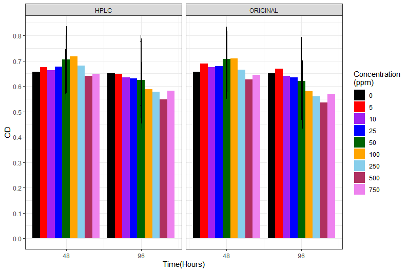
I have changed the code above for the summary, but I am in trouble with why are the "SDs" are just on the green bars.

library(ggplot2)
library(dplyr)

AptaC10run123<-(read.csv("~/R/Data Analysis/MSc ARTs/Summary/June 2022/AptataC10RawPur.4896H.csv", stringsAsFactors=TRUE))

AptaC10 <- aggregate(bgrowth ~ con + time + Purification, AptaC10run123,mean)

summary<-AptaC10run123 %>%
group_by(time, con, Purification) %>%
get_summary_stats(bgrowth, type = "mean_sd")
data.frame(summary)

summary <- summary |> mutate(mean=as.numeric(mean),
con=formatC(as.numeric(con),width=3,flag = "0"))
ggplot(data = summary, mapping = aes(x=time, y=mean, fill=con)) +
geom_bar(stat="identity", position = "dodge") +
geom_errorbar(aes(ymin=mean-sd, ymax=mean+sd, group=con),size=.5, width=.2,
position=position_dodge(.9))+

facet_grid(~Purification)+
theme_bw()+
scale_fill_manual(name = "Concentration\n(ppm)",
values = c("000" = "black", "005" = "red", "010"= "purple",
"025"="blue", "050"= "darkgreen", "100"= "orange",
"250"= "skyblue", "500"="maroon", "750"="violet"),
labels=c("0","5","10","25","50","100","250","500","750")) +

scale_y_continuous(breaks = seq(0,1, by=0.1)) +
scale_x_continuous(breaks= seq(0,96, by=48))+
xlab("Time(Hours)")+
ylab("OD")

Please post the output of

dput(summary)

so others can easily work with the data you are plotting.

@FJCC , You mean this one,

data.frame(summary)
time con Purification variable n mean sd
1 48 000 HPLC bgrowth 3 0.657 0.089
2 48 000 ORIGINAL bgrowth 3 0.657 0.089
3 48 005 HPLC bgrowth 3 0.674 0.128
4 48 005 ORIGINAL bgrowth 3 0.689 0.136
5 48 010 HPLC bgrowth 3 0.663 0.107
6 48 010 ORIGINAL bgrowth 3 0.675 0.125
7 48 025 HPLC bgrowth 3 0.676 0.123
8 48 025 ORIGINAL bgrowth 3 0.678 0.126
9 48 050 HPLC bgrowth 3 0.705 0.131
10 48 050 ORIGINAL bgrowth 3 0.708 0.127
11 48 100 HPLC bgrowth 3 0.717 0.105
12 48 100 ORIGINAL bgrowth 3 0.709 0.108
13 48 250 HPLC bgrowth 3 0.681 0.080
14 48 250 ORIGINAL bgrowth 3 0.664 0.079
15 48 500 HPLC bgrowth 3 0.640 0.045
16 48 500 ORIGINAL bgrowth 3 0.626 0.048
17 48 750 HPLC bgrowth 3 0.649 0.044
18 48 750 ORIGINAL bgrowth 3 0.645 0.053
19 96 000 HPLC bgrowth 3 0.651 0.125
20 96 000 ORIGINAL bgrowth 3 0.651 0.125
21 96 005 HPLC bgrowth 3 0.648 0.152
22 96 005 ORIGINAL bgrowth 3 0.669 0.150
23 96 010 HPLC bgrowth 3 0.635 0.144
24 96 010 ORIGINAL bgrowth 3 0.641 0.152
25 96 025 HPLC bgrowth 3 0.631 0.158
26 96 025 ORIGINAL bgrowth 3 0.635 0.158
27 96 050 HPLC bgrowth 3 0.625 0.163
28 96 050 ORIGINAL bgrowth 3 0.621 0.155
29 96 100 HPLC bgrowth 3 0.589 0.136
30 96 100 ORIGINAL bgrowth 3 0.579 0.125
31 96 250 HPLC bgrowth 3 0.577 0.115
32 96 250 ORIGINAL bgrowth 3 0.559 0.110
33 96 500 HPLC bgrowth 3 0.547 0.114
34 96 500 ORIGINAL bgrowth 3 0.536 0.119
35 96 750 HPLC bgrowth 3 0.581 0.115
36 96 750 ORIGINAL bgrowth 3 0.567 0.135

Using position_dodge2() seems to work.

summary <- read.csv("~/R/Play/Dummy.csv", sep = " ")
library(ggplot2)
library(dplyr)
#> 
#> Attaching package: 'dplyr'
#> The following objects are masked from 'package:stats':
#> 
#>     filter, lag
#> The following objects are masked from 'package:base':
#> 
#>     intersect, setdiff, setequal, union
summary <- summary |> mutate(mean=as.numeric(mean),
                             con=formatC(as.numeric(con),width=3,flag = "0"))

ggplot(data = summary, 
       mapping = aes(x=time, y=mean, ymin=mean-sd, ymax=mean+sd, 
                     fill=con)) +
  geom_bar(stat="identity", position = position_dodge()) +
  geom_errorbar(size=.5, #group=con width=.2
                position=position_dodge2(.9))+
  
  facet_grid(~Purification)+
  theme_bw()+
  scale_fill_manual(name = "Concentration\n(ppm)",
                    values = c("000" = "black", "005" = "red", "010"= "purple",
                               "025"="blue", "050"= "darkgreen", "100"= "orange",
                               "250"= "skyblue", "500"="maroon", "750"="violet"),
                    labels=c("0","5","10","25","50","100","250","500","750")) +
  
  scale_y_continuous(breaks = seq(0,1, by=0.1)) +
  scale_x_continuous(breaks= seq(0,96, by=48))+
  xlab("Time(Hours)")+
  ylab("OD")

Created on 2022-07-03 by the reprex package (v2.0.1)

This topic was automatically closed 21 days after the last reply. New replies are no longer allowed.

If you have a query related to it or one of the replies, start a new topic and refer back with a link.