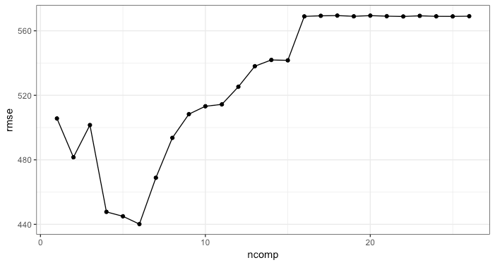
Here's a tidy workflow that I used to see if estimating the transformations inside of resampling made a big difference (it didn't):
library(recipes)
library(rsample)
library(yardstick)

# create the recipe without the formula to more easily
pls_rec <- recipe(total_N2O ~ ., data = annual_flux) %>%
  add_role(series, town, avg_N2O, log_avg_N2O,year, log_total_N2O,
           new_role = "other data") %>%
  step_YeoJohnson(all_predictors()) %>%
  step_center(all_predictors()) %>%
  step_scale(all_predictors())

# functions to fit the model and get predictions + RMSE
pls_fit <- function(recipe, ...) {
  plsr(total_N2O ~ ., data = juice(recipe, all_predictors(), all_outcomes()))
}
pls_pred <- function(split, recipe, model, ...) {
  # get the holdout data via `assessment` then preprocess
  pred_data <- bake(recipe, newdata = assessment(split), all_predictors(), all_outcomes())

  # One outcome so drop the dimension to a 2d array
  pred_vals <- predict(model, newdata = pred_data)[,1,] %>%
    as.data.frame() %>%
    bind_cols(assessment(split) %>% select(total_N2O)) %>%
    # drop the predictions per component into a long df
    gather(label, prediction, -total_N2O) %>%
    # convert "X comp" to a numeric X
    mutate(
      ncomp = gsub(" comps", "", label),
      ncomp = as.numeric(ncomp)
      ) %>%
    # add resampling labels
    cbind(labels(split))
}


# setup a resampling scheme, estimate the recipes, fit the models and
# make predictions,
set.seed(57256)
folds <- vfold_cv(annual_flux, repeats = 5) %>%
  mutate(
    recipes = map(splits, prepper, pls_rec, retain = TRUE),
    models = map(recipes, pls_fit, validation = "none"),
    pred = pmap(
      list(split = splits, recipe = recipes, model = models),
      pls_pred
    )
  )

# get the RMSE values, summarize by #comps and plot

pred_vals <- folds %>%
  pull(pred) %>%
  bind_rows()

performance <- pred_vals %>%
  group_by(ncomp, id, id2) %>%
  do(metrics(., truth = total_N2O, estimate = prediction))

av_performance <- performance %>%
  group_by(ncomp) %>%
  summarize(rmse = mean(rmse), rsq = mean(rsq))

ggplot(av_performance, aes(x = ncomp, y = rmse)) +
  geom_point() +
  geom_line() +
  theme_bw()
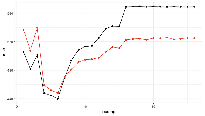
We can compare this to what comes out of plsr (very similar pattern) via
# compare to orignal objects
original_pls_model <-
  data.frame(
    ncomp = 0:26,
    rmse = unname(RMSEP(plsFit)$val[1,1,]),
    rsq = unname(R2(plsFit)$val[1,1,])
  ) %>%
  filter(ncomp > 0)

# pretty consistent with the original model; values are different due
# to different resamples (and more too)
ggplot(av_performance, aes(x = ncomp, y = rmse)) +
  geom_point() +
  geom_line() +
  geom_point(data = original_pls_model, col = "red") +
  geom_line(data = original_pls_model, col = "red") +
  theme_bw()

