Approximation of a function of two variables - 3D surface

[nickcin]

I have measurement results at several points with coordinates in the form of a table - latitude, longitude, value. It is necessary 1) to construct an approximating surface. 2) get the value at a point with given coordinates. Of course, it would be better to do this in a geographical projection, but it can also be calculated in the Cartesian system, because the coordinates are close. What is the easiest way to do this in Rstudio? I tried a dozen ways - absolutely nothing worked. In all cases, functions like surface3d, interp.surface, loess and the like do something that is not what is required, the wrong parameters. I haven't found any suitable function to solve this problem. It seemed to me that it should be very simple.

[quantoid]

I would estimate a generalized additive model of the measurement on the smoothed interaction of latitude and longitude). You could then use a grid to plot the surface and put the points there as well with either persp() or wireframe() or with plotly(). If you need more direction, upload some data and we can go from there.

[nickcin]

Thank you for responding and deciding to help. Here is the table. Copy to csv-file and use.
|M|X|Y|Z|
|Station1|37.5305555555556|56.6675|100.0000000000000|
|Station2|35.6716666666667|56.4219444444444|100.0000000000000|
|Station3|39.1044444444444|55.8358333333333|98.5294117647059|
|Station4|36.5108333333333|55.7591666666667|93.6170212765957|
|Station5|36.9611111111111|55.5833333333333|96.0176991150443|
|Station6|38.5930555555556|54.5727777777778|0.0000000000001|
|Station7|38.475|54.5147222222222|62.962962962963|
|Station8|38.5286111111111|54.4002777777778|7.69230769230769|

[quantoid]

Let's start by making the data.

dat <- tibble::tribble(~M, ~X, ~Y, ~Z, 
"Station1", 37.5305555555556, 56.6675, 100.0000000000000, 
"Station2", 35.6716666666667, 56.4219444444444, 100.0000000000000, 
"Station3", 39.1044444444444, 55.8358333333333, 98.5294117647059, 
"Station4", 36.5108333333333, 55.7591666666667, 93.6170212765957, 
"Station5", 36.9611111111111, 55.5833333333333, 96.0176991150443, 
"Station6", 38.5930555555556, 54.5727777777778, 0.0000000000001, 
"Station7", 38.475, 54.5147222222222, 62.962962962963, 
"Station8", 38.5286111111111, 54.4002777777778, 7.69230769230769)

Netxt, we can load the mgcv package and estimate the model - you want a smoothed interaction between X and Y predicting Z. If the surface is not sufficiently close to the points, you can change the k argument in te() and ti(), which will change the dimensions of the basis functions used in the GAM. Bigger values mean functions that are more flexible.

library(mgcv)
#> Loading required package: nlme
#> This is mgcv 1.9-0. For overview type 'help("mgcv-package")'.
g <- gam(Z ~ te(X) + te(Y) + ti(X,Y), data=dat)

Depending on how you want to plot the output, you will need the predictions in different formats. First, let's define the grid points we'll use to evaluate the model and plot the surface. I chose 50 evenly spaced points across the ranges of X and Y.

x_seq = seq(min(dat$X), max(dat$X), length=50)
y_seq = seq(min(dat$Y), max(dat$Y), length=50)

If you're using wireframe() from the lattice package, you'll need the data in long format where the columns of X and Y represent all possible combinations of the X and Y values and then Z is the fitted values from the model at those values of X and Y. I find the wireframe plots difficult to manipulate to get the right view and there will be some added extra work to get the original points in the space too.

## Wireframe
ll_grid <- expand.grid(X = x_seq, 
                       Y = y_seq)

ll_grid$fit <- predict(g, newdata=ll_grid)
library(lattice)
wireframe(fit ~ X + Y, data=ll_grid, drape=TRUE)

You mentioned wanting to be able to generate a prediction for any particular (X,Y) pair, you can do that easily with:

predict(g, newdata=data.frame(X=55, Y=37))
#>        1 
#> -10852.1

For persp() or plot_ly() you'll need the fitted values in a different format. Specifically, you'll need a matrix where each cell represents the prediction at one X and one Y value. The easiest way is to make a little function that will generate predictions for an x-y pair and then use outer() to loop over the unique values of X and Y

predict_g <- function(x,y){
  predict(g, newdata=data.frame(X=x, Y=y))
}

predict_g(55, 37)
#>        1 
#> -10852.1


fit <- outer(x_seq, y_seq, predict_g)

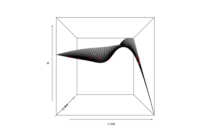
Then, you can make the perspective plot with the following (note, the theta parameter rotates the plot in the horizontal direction and phi in the vertical direction):

p <- persp(x_seq, y_seq, fit)

If you want to add the points in, you an translate them into the same 2-D space with trans3d() and the output from the original perspective plot. Then add them in with points().

new_xy <- trans3d(dat$X, dat$Y, dat$Z, pmat=p)
points(new_xy$x, new_xy$y, pch=16, col="red")

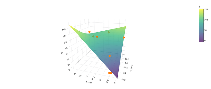
Another option is to use plotly - a package that makes interactive graphics. One great thing is that it uses data in the same format as persp() and is even easier to incorporate the points:

library(plotly)

plot_ly() %>% 
  add_surface(x=~x_seq, y=~y_seq, z=t(fit), alpha=.75) %>% 
  add_markers(data=dat, x=~X, y=~Y, z=~Z)

The plot below is a screenshot of the output, but the output is interactive - in that you can spin it around with your cursor. You could also put tooltip identifiers on the points if you wanted. There are lots of options here:

^{Created on 2024-02-26 with reprex v2.0.2}

[nickcin]

Excellent, just what you need! Thanks a lot! I'll try it myself now.

You need to swap the values 55 and 37, then z will be normal 0<=z<=100:
X - longitude (37)
Y - latitude (55)

It is necessary to set boundary conditions z - these are percentages from 0 to 100
At both boundaries there is an exponential approach to 0 or 100

I only get the second graph, but the first and third ones are not displayed

[nickcin]

Why might the first and last graphs not be displayed?
Libraries installed and loaded
Doesn't write any errors

If me deliberately make a error in the arguments, it throws an error at runtime. Those. The code is executed, but the graph is not displayed.

[quantoid]

Not sure why the other graphs do not display. They worked for me as you saw.

[nickcin]

Added a new point.
"Station9", 35.4788888888889, 55.5172222222222, 100.0000000000000

And turned the graph.
p <- persp(x_seq, y_seq, fit, theta = 0, phi = 0)

I don’t really like the result, something is wrong.
No differences are visible from 0 to 100 in height.

[nickcin]

The spline oscillates too much. Is there a way to achieve data shape preservation?

[quantoid]

What do you mean by "data shape preservation"?

[nickcin]

This means maintaining monotony, as well as convexity, concavity, and quasilinearity in all areas between reference points, depending on the data. And I would also like to add parameters for the GAM so that the function does not go beyond the boundaries of Z.

[nirgrahamuk]

I don't have time to work on a detailed application to your issue; but im fairly confident you can make a good approximate surface of arbitrary precision with interp package CRAN - Package interp

[quantoid]

If you like the GAM approach, there is a package called "scam" (shape constrained additive models) that has bivariate smoothers with monotonicity constraints or univariate monotone smoothers with convexity/concavity constraints.

[nickcin]

Thanks for the advice! Very interesting, this seems to be what me need!